Sailco, a simple example #

Sailco manufactures sailboats. During the next 4 months the company must meet the following demands for their sailboats:

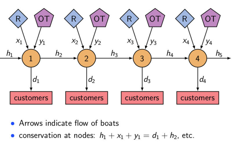
At the beginning of Month 1, Sailco has 10 boats in inventory. Each month it must determine how many boats to produce. During any month, Sailco can produce up to 40 boats with regular labor and an unlimited number of boats with overtime labor. Boats produced with regular labor cost 400 USD each to produce, while boats produced with overtime labor cost 450 USD each. It costs 20 USD to hold a boat in inventory from one month to the next. Find the production and inventory schedule that minimizes the cost of meeting the next 4 months’ demands

using JuMP, HiGHS, DataStructures, NamedArrays

Solution #

m = Model(HiGHS.Optimizer)

demands = [40, 60, 70, 25]

# boats built with regular labor
@variable(m, 0 <= x[1:4] <= 40)
# boats built with overtime labor
@variable(m, y[1:4] >= 0)
# inventory
@variable(m, h[1:5] >= 0)

# for each month
for i in range(1,4)
#     boats plus the inventory must be larger than the demand
#     @constraint(m, x[i] + y[i] + h[i] >= demands[i])
    
    # inventory next month is equal to all boats available minus the demand of that month
    @constraint(m, h[i+1] == h[i] + x[i] + y[i] - demands[i])
end

# first month inventory is 10
@constraint(m, h[1] == 10)

# minimize the total cost
@objective(m, Min, 400*sum(x) + 450*sum(y) + 20*sum(h))

optimize!(m)
println("Solver terminated with status ", termination_status(m))

Running HiGHS 1.4.2 [date: 1970-01-01, git hash: f797c1ab6]
Copyright (c) 2022 ERGO-Code under MIT licence terms
Presolving model
4 rows, 12 cols, 15 nonzeros
4 rows, 12 cols, 15 nonzeros
Presolve : Reductions: rows 4(-1); columns 12(-1); elements 15(-2)
Solving the presolved LP
Using EKK dual simplex solver - serial
  Iteration        Objective     Infeasibilities num(sum)
          0     2.0000000000e+02 Pr: 4(185) 0s
          5     7.6400000000e+04 Pr: 0(0) 0s
Solving the original LP from the solution after postsolve
Model   status      : Optimal
Simplex   iterations: 5
Objective value     :  7.6400000000e+04
HiGHS run time      :          0.00
Solver terminated with status OPTIMAL

println("Boats built with regular labor each month: ", Array{Int}(value.(x)))
println("Boats built with overtime labor each month: ", Array{Int}(value.(y)))
println("Inventory: ", Array{Int}(value.(h)))
println("Minimum cost: \`$", objective_value(m))

Boats built with regular labor each month: [40, 40, 40, 25]
Boats built with overtime labor each month: [0, 10, 30, 0]
Inventory: [10, 10, 0, 0, 0]
Minimum cost: $`76400.0

In above,

# for each month
for i in range(1,4)
    # inventory next month is equal to all boats available minus the demand of that month
    @constraint(m, h[i+1] == h[i] + x[i] + y[i] - demands[i])
end

can be rewritten as

@constraint(m, flows[i in 1:4], h[i] + x[i] + y[i] == demands[i] + h[i])

Minimum-cost flow problem #

Lumber transportation problem (J. Reeb and S. Leavengood) #

Millco has three wood mills and is planning three new logging sites. Each mill has a maximum capacity and each logging site can harvest a certain number of truckloads of lumber per day. The cost of a haul is 2 USD/mile of distance. If distances from logging sites to mills are given below, how should the hauls be routed to minimize hauling costs while meeting all demands?

m = Model(HiGHS.Optimizer)

sites = [1, 2, 3]
mills = [:A, :B, :C]

cost_per_haul = 4

supply = Dict(zip(sites, [20, 30, 45]))
demand = Dict(zip(mills, [30, 35, 30]))

dist = NamedArray([8 15 50; 10 17 20; 30 26 15], (sites, mills), ("Sites", "Mills"))

3×3 Named Matrix{Int64}
Sites ╲ Mills │ :A  :B  :C
──────────────┼───────────
1             │  8  15  50
2             │ 10  17  20
3             │ 30  26  15

@variable(m, x[sites, mills] >= 0)

@constraint(m, sup[i in sites], sum(x[i,j] for j in mills) == supply[i])
@constraint(m, dem[j in mills], sum(x[i,j] for i in sites) == demand[j])
@objective(m, Min, cost_per_haul * sum( x[i,j]*dist[i,j] for i in sites, j in mills ))

optimize!(m)

Running HiGHS 1.4.2 [date: 1970-01-01, git hash: f797c1ab6]
Copyright (c) 2022 ERGO-Code under MIT licence terms
Presolving model
6 rows, 9 cols, 18 nonzeros
5 rows, 9 cols, 15 nonzeros
Presolve : Reductions: rows 5(-1); columns 9(-0); elements 15(-3)
Solving the presolved LP
Using EKK dual simplex solver - serial
  Iteration        Objective     Infeasibilities num(sum)
          0     0.0000000000e+00 Pr: 5(155) 0s
          5     5.7600000000e+03 Pr: 0(0) 0s
Solving the original LP from the solution after postsolve
Model   status      : Optimal
Simplex   iterations: 5
Objective value     :  5.7600000000e+03
HiGHS run time      :          0.00

NamedArray(Int[value(x[i,j]) for i in sites, j in mills], (sites, mills), ("Sites", "Mills"))

3×3 Named Matrix{Int64}
Sites ╲ Mills │ :A  :B  :C
──────────────┼───────────
1             │  0  20   0
2             │ 30   0   0
3             │  0  15  30

Swim relay problem (Van Roy and Mason) #

The coach of a swim team needs to assign swimmers to a 200-yard medley relay team to compete in a tournament. The problem is that his best swimmers are good in more than one stroke, so it’s not clear which swimmer to assign to which stroke. Here are the best times for each swimmer:

This can be considered as a transportation problem like the Lumber transportation problem we talked about above.

m = Model(HiGHS.Optimizer)

strokes = [:ackstroke, :breaststroke, :butterfly, :freestyle]
persons = [:carl, :chris, :david, :tony, :ken]

speed = NamedArray(
    [
        37.7 32.9 33.8 37 35.4; 
        43.4 33.1 42.2 34.7 41.8;
        33.3 28.5 38.9 30.4 33.6;
        29.2 26.4 29.6 28.5 31.1 
        ], (strokes, persons), ("Stroke", "Person"))

supply = Dict(zip(strokes, [1,1,1,1]))

@variable(m, x[strokes, persons] >= 0)

# each person should swim at most once
@constraint(m, swimmer[p in persons], sum(x[s, p] for s in strokes) <= 1)

# each stroke should be assigned to exactly one person
@constraint(m, assignment[s in strokes], sum(x[s, p] for p in persons) == 1)

# minimize the time consumed
@objective(m, Min, sum(x[s, p] * speed[s,p] for s in strokes, p in persons))

optimize!(m)

Running HiGHS 1.4.2 [date: 1970-01-01, git hash: f797c1ab6]
Copyright (c) 2022 ERGO-Code under MIT licence terms
Presolving model
9 rows, 20 cols, 40 nonzeros
9 rows, 20 cols, 40 nonzeros
Presolve : Reductions: rows 9(-0); columns 20(-0); elements 40(-0) - Not reduced
Problem not reduced by presolve: solving the LP
Using EKK dual simplex solver - serial
  Iteration        Objective     Infeasibilities num(sum)
          0     0.0000000000e+00 Pr: 4(4) 0s
          8     1.2620000000e+02 Pr: 0(0) 0s
Model   status      : Optimal
Simplex   iterations: 8
Objective value     :  1.2620000000e+02
HiGHS run time      :          0.00

NamedArray([value(x[s,p]) for s in strokes, p in persons], (strokes, persons), ("Stroke", "Person"))

4×5 Named Matrix{Float64}
Stroke ╲ Person │  :carl  :chris  :david   :tony    :ken
────────────────┼───────────────────────────────────────
:ackstroke      │    0.0     0.0     1.0     0.0     0.0
:breaststroke   │    0.0     0.0     0.0     1.0     0.0
:butterfly      │    0.0     1.0     0.0    -0.0     0.0
:freestyle      │    1.0    -0.0     0.0     0.0     0.0

Last modified on 2023-03-17