PID controller #
PID is short for “Proportional-Integral-Derivative”. What it does is that if you have a planned trajectory for a vehicle which is now at a specific location and have a specific initial speed, PID will allow this vehicle to get to the planned trajectory. You accomplish this through PID by tweaking the three parameters:
$k_P$$k_I$$k_D$
If you multiply $k_P$ by the distance between the planned location and the actual location at any timestamp, you get $a_P$. If you multiply $k_I$ by the difference between the integral of the planned location and that of the actual location at any timestamp, you get $a_I$. If you multiply $k_D$ by the speed difference between the planned trajectory and the actual vehicle at any timestamp, you get $a_D$.
If you add up $a_P$, $a_I$, and $a_D$, you get $a$, which is the acceleration for the actual vehicle.
PID for constant speed #
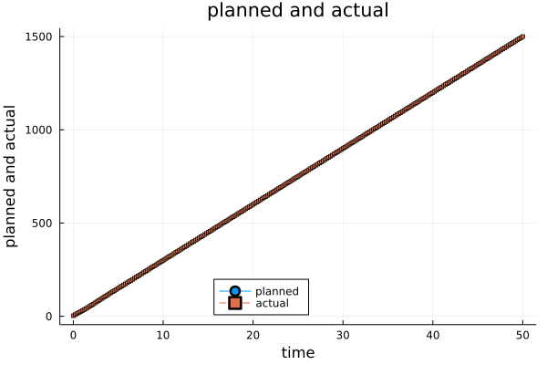
The planned trajectory starts from location 0 at time 0. It is cruising at 30m/s speed for 50 seconds.The actual location is 3 at time 0 and the actual speed is 28m/s at time 0.
using Plots, Distributions, Random
function get_data(t, k_p=2, k_i=0, k_d=1)
    # initial state
    # y for the planned vehicle, x for the actual vehicle

    y = 0 # position
    int_y = 0 # integral of position
    y_dot = 30 # speed
    x = 3
    int_x = 0
    x_dot = 28

    a_p = k_p * (y - x)
    a_i = k_i * (int_y - int_x)
    a_d = k_d * (y_dot - x_dot)

    a = a_p + a_i + a_d

    # if time is 0, return the initial state
    if t == 0
        return (y, x)
    else
        for i in time_delta:time_delta:t
            # 0.2, 0.4, 0.6, ...
            x_dot_prev = x_dot
            x_dot += a * time_delta
            # THIS IS USING APPROXIMATION!
            x += 0.5*(x_dot_prev + x_dot) * time_delta
            int_x += x * time_delta

            # update y
            y_dot = y_dot # constant speed at all time
            y += y_dot * time_delta
            int_y += y * time_delta

            # update a_p, a_i, a_d, and a for usage at next timestamp
            a_p = k_p * (y - x)
            a_i = k_i * (int_y - int_x)
            a_d = k_d * (y_dot - x_dot)
            a = a_p + a_i + a_d
        end
        return (y, x)
    end
end
get_data (generic function with 5 methods)
time_delta = 0.2
time_span = 0.0:time_delta:50
0.0:0.2:50.0
function make_plot(data, title, label, xlabel, ylabel)
    Plots.plot(time_span, data,
    title=title,
    label=label,
    linewidth=0.5,
    markershape = :auto,
    markersize = 2,
    linestyle = :auto,
    mc= :auto,
    xlabel = xlabel,
    ylabel = ylabel,
    legend=:bottom
    )
end
make_plot (generic function with 1 method)
ys = [get_data(i, 2, 0, 1)[1] for i in time_span]
xs = [get_data(i, 2, 0, 1)[2] for i in time_span]
251-element Vector{Real}:
    3
    8.52
   13.915199999999999
   19.253951999999998
   24.59818752
   29.999490355200003
   35.496625508352004
   41.114488996331524
   46.8643352065278
   52.745059206570446
   58.74526263008063
   64.84581249542273
   71.02260938267628
    ⋮
 1434.0000000008072
 1440.0000000013742
 1446.0000000017405
 1452.000000001909
 1458.000000001898
 1464.0000000017367
 1470.0000000014622
 1476.0000000011148
 1482.0000000007337
 1488.000000000355
 1494.0000000000084
 1499.9999999997167
make_plot(
    [ys, xs],
    "planned and actual",
    ["planned" "actual"],
    "time",
    "planned and actual"
)

savefig("/en/blog/2023-02-28-pid_files/pid-01.png")
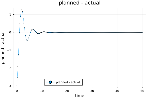
make_plot(
    ys-xs,
    "planned - actual",
    "planned - actual",
    "time",
    "planned - actual"
)

savefig("/en/blog/2023-02-28-pid_files/pid-02.png")
Dynamic speed (with random noise) #
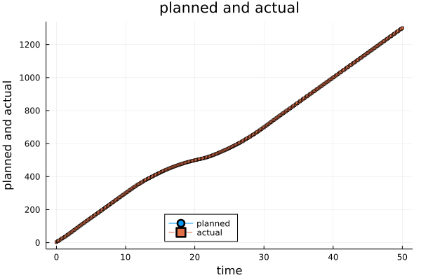
The planned trajectory starts from location 0 at time 0. It is cruising at 30m/s speed for the first 10 seconds, then decreasing to 10 m/s with deceleration
$-2𝑚/𝑠^2$for 10 seconds and then accelerating to 30m/s with acceleration$2𝑚/𝑠^2$for 10 seconds, and then cruising at 30 m/s for 20 seconds.
The actual location is 3 at time 0 and the actual speed is 28m/s at time 0.
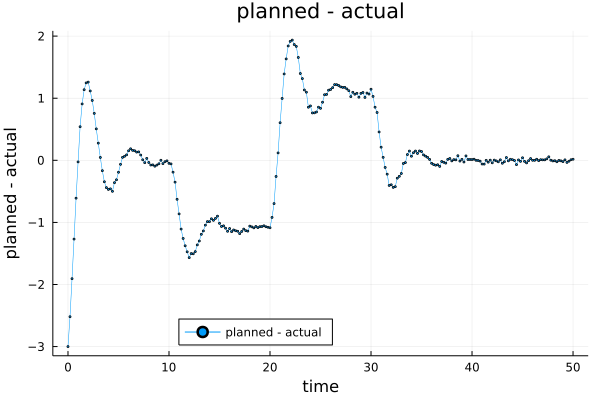
Assuming the acceleration cannot be precisely controlled, and always has a random error uniformly distributed over
$[-0.2, 0.2] m/s$
function get_y_dot(t)
    """This function gets the speed of the planned vehicle
    """
    if t <= 10
        y_dot = 30
    elseif t <= 20
        y_dot = 30
        for i in 10+time_delta:time_delta:t
            y_dot += time_delta*(-2)
        end
    elseif t <= 30
        y_dot = 10
        for i in 20+time_delta:time_delta:t
            y_dot += time_delta*2
        end
    else
        y_dot = 30
    end
    return y_dot
end
get_y_dot (generic function with 1 method)
Tesing the function of get_y_dot:
get_y_dot(15)
20.000000000000036
get_y_dot(22)
14.000000000000004
function get_data(t, k_p=2, k_i=0, k_d=1, noise = true)
    """This function returns the trajectory of the planned vehicle (y)
    and the actual vehicle (x)

    The key is that the initial acceleration of the actual vehicle can be calculated
    through the initial state and the set parameters. Using this acceleration at t=0,
    we can calculate the velocity of the actual vehicle at the next timestamp. Then,
    using x_dot, we can calculate x and int_x.

    y_dot, y, and the int_y can be calculated easily.
    """
    # initial state
    # y for the planned vehicle, x for the actual vehicle

    y = 0 # position
    int_y = 0 # integral of position
    y_dot = 30 # speed
    x = 3
    int_x = 0
    x_dot = 28

    a_p = k_p * (y - x)
    a_i = k_i * (int_y - int_x)
    a_d = k_d * (y_dot - x_dot)
    if noise
        a = a_p + a_i + a_d + rand(Uniform(-0.2, 0.2))
    else
        a = a_p + a_i + a_d
    end
    if t == 0
        return (y, x)
    else
        for i in time_delta:time_delta:t
            x_dot_prev = x_dot
            x_dot += a * time_delta
            # THIS IS USING APPROXIMATION!
            x += 0.5*(x_dot_prev + x_dot) * time_delta
            int_x += x * time_delta

            # update y
            y_dot = get_y_dot(i)
            y += y_dot * time_delta
            int_y += y * time_delta

            # update a_p, a_i, a_d, and a for usage at next timestamp
            a_p = k_p * (y - x)
            a_i = k_i * (int_y - int_x)
            a_d = k_d * (y_dot - x_dot)
            if noise
                a = a_p + a_i + a_d + rand(Uniform(-0.2, 0.2))
            else
                a = a_p + a_i + a_d
            end
        end
        return (y, x)
    end
end
get_data (generic function with 5 methods)
ys = [get_data(i, 2, 0, 1)[1] for i in time_span]
xs = [get_data(i, 2, 0, 1)[2] for i in time_span]
251-element Vector{Real}:
    3
    8.518715767262622
   13.906232802166503
   19.268572854391913
   24.6096425130715
   30.02599498962064
   35.45927678410515
   41.09226062787909
   46.86326171393311
   52.7531619121299
   58.74007729213587
   64.88326196481631
   71.03580647914927
    ⋮
 1233.9981479653238
 1240.010372398277
 1246.0066976688347
 1252.0239301638433
 1258.0021171428577
 1264.008764132957
 1270.021276479265
 1275.9923591224674
 1282.033955662245
 1288.014337231835
 1293.9907637632514
 1299.9826222077306
make_plot(
    [ys, xs],
    "planned and actual",
    ["planned" "actual"],
    "time",
    "planned and actual"
)

savefig("/en/blog/2023-02-28-pid_files/pid-03.png")
make_plot(
    ys-xs,
    "planned - actual",
    "planned - actual",
    "time",
    "planned - actual"
)

savefig("/en/blog/2023-02-28-pid_files/pid-04.png")
Questions #
- In pid, the x/y_dot, and int_y/x is using approximation, can we get the exact form?
It’s very difficult to get the analytical form.
- How to get the optimal value
It’s also very difficult. It involves non-linear programming.
#self-drivingLast modified on 2025-06-03 • Suggest an edit of this page