ACC-Automated Car Following Model

Hongtao Hao / 2023-02-28

The material below is based on Professor Xiaopeng Li ’s course of CIV ENGR 679 Connected and Automated Transport

This notebook runs in Julia and is rendered by Hupyter .

ACC-Automated Car Following Model #

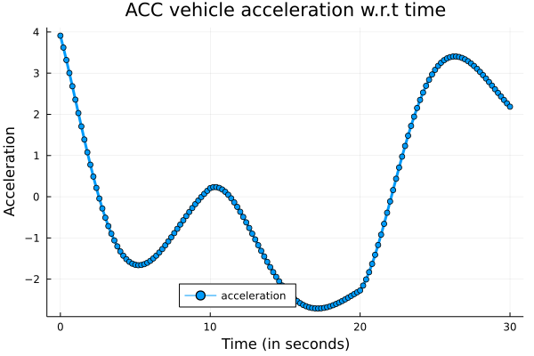
ACC is short for “Adaptive cruise control”. It is a control model based on acceleration. It has the following formula:

$$a_{AV} (t) = k_1 (g(t) - \tau v_{AV}(t)) + k_2 \Delta v$$

Functions #

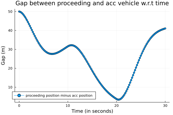
$a_{AV} (t)$ : function of the acceleration of the ACC vehicle (which is following another vehilce), with respect to time
$g(t)$ : function of the gap between the two vehicles (the position of the preceeding vehicle minus that of the ACC vehicle) with respect to time
$v_{AV}(t)$ : function of the ACC vehicle’s speed with respect to time.

Parameters #

$k_1 = 0.23 s^{-2}$ (What does $s^{-2} mean?$ )
$k_2 = 0.07 s^{-1}$
$\tau$ , safety time gap between the two vehicles

Example #

Let’s consider the following example:

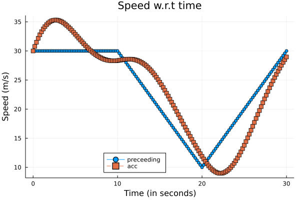
The preceding vehicle is cruising at 30m/s speed for the first 10 seconds, then decreasing to $10 m/s$ with deceleration $−2𝑚/𝑠^2$ and then accelerating to 30m/s with acceleration $2𝑚/𝑠^2$ . The initial speed of the following ACC vehicle is 30m/s.

$\tau = 1.1s$

Initial spacing is $20m$

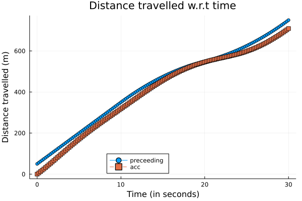
Based on the above settings, we want to plot the trajectory of the two vehhicles.

using Plots

# Planned Trajectory
v_cruise = 30 # m/s
t_cruise = 10 # first 10 seconds
a_decel = -2   # m/s^2
a_accel = 2    # m/s^2
init_space = 50 # initial spacing is 50 m
init_acc_v = 30 # initial acc speed is 20 m/s

k1 = 0.23
k2 = 0.07 

# speed when deceleration stops
v_decel_end = 10

# how much time the preceeding vehicle decelerates
t_decel = (v_cruise - v_decel_end)/abs(a_decel) 

# speed when deceleration stops
v_accel_end = 30

# how much time the preceeding vehicle accelerates
t_accel = (v_accel_end - v_decel_end)/abs(a_accel) 

time_interval = 0.2
time_span = 0.0:time_interval:30

safety_time_gap = 1.1

1.1

function traj(t)
    """This function defines the trajectory of the preceeding vehicle
    
        - v_p: the speed of the preceeding vehicle
        - x_p: the distance the preceeding vehicle has travelled
    """
    if t <= t_cruise
        
        v_p = v_cruise
        x_p = init_space + v_cruise * t
    elseif t <= t_cruise + t_decel
        v_p = v_cruise + a_decel * (t - t_cruise)
        # I used calculs to do this:
        # from 10s to 20s, the speed w.r.t time is v(t) = 30 - 2t
        # The integral of v(t) is the distance w.r.t time: S(t) = -t^2 + 30t + c
        # since S(0) = 0, so c = 0
        # therefore, S(t) = -t^2 + 30t
        
        # to be more general, 30 should be v_cruise here
        x_p = init_space + v_cruise * t_cruise - (t-t_cruise)^2 + v_cruise * (t - t_cruise)
    elseif t <= t_cruise + t_decel + t_accel
        v_p = v_decel_end + a_accel * (t - t_cruise - t_decel)
        # I used calculs to do this:
        # from 20s to 30s, the speed w.r.t time is v(t) = 10 + 2t
        # The integral of v(t) is the distance w.r.t time: S(t) = t^2 + 10t + c
        # since S(0) = 0, so c = 0
        # therefore, S(t) = t^2 + 10t
        
        # to be more general, 10 should be v_decel_end here
        x_p = init_space + v_cruise * t_cruise - t_decel^2 + v_cruise * t_decel + (
            t - t_cruise - t_decel)^2 + v_decel_end * (t - t_cruise - t_decel)
    end
    return (v_p, x_p)
end

traj (generic function with 1 method)

function traj_acc(t, safety_time_gap = safety_time_gap)
    """This function definds the trajectory of the acc vehicle
    """
    # initialize at timestamp 0.0
    v_p, x_p = traj(0)
    x_av = 0
    v_av = init_acc_v
    a_av = k1*((x_p - x_av) - safety_time_gap*v_av) + k2 * (v_p - v_av)
    
    # if t == 0, return the initial result
    if t == 0
        return (x_av, v_av, a_av)
    # otherwise, use for loop for calculation
    else
        for i in time_interval:time_interval:t
            # the first is 0.2, then 0.4, 0.6...
            v_p, x_p = traj(i)
            
            # calculate
            v_av_prev = v_av
            v_av += time_interval*a_av
            ## HOW?
            x_av += 0.5*(v_av + v_av_prev)*time_interval + time_interval^2 * 0.5*a_av
            a_av = k1*((x_p - x_av) - safety_time_gap*v_av) + k2 * (v_p - v_av)
            
        end
        # return the results

        return (x_av, v_av, a_av)
    end
end

traj_acc (generic function with 2 methods)

function make_plot(data, title, label, xlabel, ylabel)
    """A helper function to make plots
    """
    Plots.plot(time_span, data,
    title=title,
    label=label,
    linewidth=3,
    markershape = :auto,
    linestyle = :auto,
    mc= :auto,
    xlabel = xlabel,
    ylabel = ylabel,
    legend=:bottom, legendcolumns=3
    )
end

make_plot (generic function with 1 method)

# speed of preceeding vehicles
vps = [traj(t)[1] for t in time_span]
# distance of preceeding vehicles
xps = [traj(t)[2] for t in time_span]

# distance, speed, and acceleration of the acc vehicle
x_av = [traj_acc(t, 1.1)[1] for t in time_span]
v_av = [traj_acc(t, 1.1)[2] for t in time_span]
a_av = [traj_acc(t, 1.1)[3] for t in time_span]

make_plot(
    [xps, x_av],
    "Distance travelled w.r.t time",
    ["preceeding" "acc"],
    "Time (in seconds)",
    "Distance travelled (m)"
)
savefig("/en/blog/2023-02-28-acc_files/acc-01.png")

make_plot(
    [xps - x_av],
    "Gap between proceeding and acc vehicle w.r.t time",
    "proceeding position minus acc position",
    "Time (in seconds)",
    "Gap (m)"
)

savefig("/en/blog/2023-02-28-acc_files/acc-02.png")

make_plot(
    [vps, v_av],
    "Speed w.r.t time",
    ["preceeding" "acc"],
    "Time (in seconds)",
    "Speed (m/s)"
)

savefig("/en/blog/2023-02-28-acc_files/acc-03.png")

make_plot(
    a_av,
    "ACC vehicle acceleration w.r.t time",
    "acceleration",
    "Time (in seconds)",
    "Acceleration"
)

savefig("/en/blog/2023-02-28-acc_files/acc-04.png")

What I do not understand #

k1, k2

Think about the units. You’ll understand why k1 is $s^{-2}$ and k2 $s^{-1}$

how to calculate x_av

Use the quadratic function. If the initial velocity is $v1$ and the acceleration is $a$ , from t = 0 to t = t, the distance travelled is $v1\cdot t + 0.5\cdot a \cdot t^2$

responsive planning, how to calculate a_ac

Identify two spots (the initial one and the critical one). Then use two functions to simulate the curves.

how to always keep the safety time gap

You don’t have to.

how to get the exact distance (x_av) function w.r.t time for ac? I know probably we need to use calculs again. But it’s difficult because we need v_av in the function of x_av, and we need a_av in the function of v_av. However, we need v_av also in the function of a_av

It’s very difficult to get the analytical form.

#self-driving

Last modified on 2023-03-02