这篇教程中,我们要手写一个神经网络,其目的是识别 mnist 数字。在看这篇之前,我建议你把 逻辑回归 这篇弄懂。网络的结构如下图:
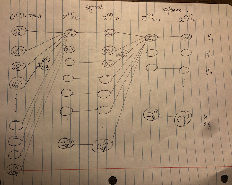
第零层是原始数据,784 个神经元,对应一张图的 784 个像素。第一层有 28 个神经元,每一个神经元对应一个抽象的「块」,比如「一个圆圈」、「左侧的一竖」、「右侧底部的一横」等等。第二层是结果,也即一张图像是 0, 1, 2, 3, … 9 的概率。
第零层所有神经元与第一层任一神经元都有连接 (权重,weight)。这是因为,第零层的神经元 (即,一个像素)对第一层的一个神经元 (一个抽象的「块」) 的意义不同。比如,底部像素对应的神经元与「右侧底部的一横」关系更紧密,因此权重更大。同样的,第一层所有神经元与第二层任一神经元都有连接,这是因为第一层神经元对于第二层神经元的意义不同。比如,「右侧底部的一横」与 0、2、3、5、9 这几个数字的关系更大,因此权重也更大。
第零层的数据导致第一层的数据,第一层的数据又导致第二层的数据。比如,手写的 3 这个数字,导致第一层「右侧底部的一横」这个神经元数值增大,这个又导致第二层与 0、2、3、5、9 相对应的神经元数值变大。
第一层的第一个神经元数据怎么算的:第零层每一个神经元的数据乘以其与第一层第一个神经元的权重,结果再加上第一层的第一个神经元对应的偏差 (bias)。这样算出来的结果从负无穷到正无穷都有可能。我们需要把这个初始结果转化为我们想要的结果,这个转化的函数被称为激活函数 (activation function)。第零层到第一层之间我们选用 sigmoid 函数。第一层到第二层我们选用 softmax 函数,因为我们最终要的结果是 10 个概率,其和为 1,softmax 函数可以实现这一点。
接下来我们需要统一一下数学表达式。
$a^{(i)}_j$表示第$i$层的第$j$个神经元。$z^{(i)}_j$也一样。需要注意的是$i$、$j$都是从$0$开始计数。$w^{(i)}_{k j}$表示第$i - 1$层第$j$个神经元与第$i$层第$k$个神经元之间的权重。$b^{(i)}_j$表示第$i$层第$j$个神经元对应的偏差。$L()$表示损失函数。$y_k$表示真实结果为$k$的概率。$\sigma ()$表示 sigmoid 函数。$S()$表示 softmax 函数。$m$表示第零层神经元数量,在这里是 784。$h$表示第一层神经元数量,在这里是 28。$c$表示第二层神经元数量,在这里是 10。 我们再看一下各个变量的维度:$a^{(0)}: 784 \times 1$$w^{(1)}: 28 \times 784$$b^{(1)}: 28 \times 1$$z^{(1)}: 28 \times 1$$a^{(1)}: 28 \times 1$$w^{(2)}: 10 \times 28$$b^{(1)}: 10 \times 1$$z^{(2)}: 10 \times 1$$a^{(2)}: 10 \times 1$$y: 10 \times 1$我们有如下的数学公式:
$$z^{(1)} = w^{(1)}a^{(0)} + b^{(1)}$$
$$a^{(1)} = \sigma(z^{(1)})$$
$$z^{(2)} = w^{(2)}a^{(1)} + b^{(2)}$$
$$a^{(2)} = S(z^{(2)})$$
损失函数我们选用 cross entropy loss。其公式为:
$$L = - \sum^{c}_{k=1} y_k \log (a^{(2)}_k)$$
求导 #
dldw2 & dldb2 #
整个神经网络的目的就在于通过减小每一步损失函数的结果来调整参数 (也即 $w^{(1)}$、$b^{(1)}$、$w^{(2)}$、$b^{(2)}$),最后让损失函数结果变得非常小。当损失函数结果变小,也就意味着我们的预测结果和真实结果的差距变小。想通过调整参数来让损失变小,那我们就需要对损失函数求 (偏) 导。我们先来看一下 $L(z^{(2)}_i)$,也就是我们先看一下损失函数的变化与 $z^{(2)}$ 中任一一个数字的变化有何关系。
以下公式中,$c$ 代表最后一共有几个结果。在我们这个情况中,最后一层是 10 个结果,分别对应结果为 0-9 的概率。
$$ \begin{aligned} \frac{\partial L}{\partial z^{(2)}_i} & = \frac{\partial \left( - \sum^{c}_{k=1} y_k \log (a^{(2)}_k) \right)}{\partial z^{(2)}_i} \\ & = - \sum^{c}_{k=1} y_k \cdot \frac{\partial \log (a^{(2)}_k)}{\partial z^{(2)}_i} \\ & = - \sum^{c}_{k=1} y_k \cdot \frac{\partial \log (a^{(2)}_k)}{\partial a^{(2)}_k} \cdot \frac{\partial a^{(2)}_k}{\partial z^{(2)}_i} \\ & = - \sum^{c}_{k=1} \frac{y_k}{a^{(2)}_k} \cdot \frac{\partial a^{(2)}_k}{\partial z^{(2)}_i} \\& = - \left( \frac{y_i}{a^{(2)}_i} \cdot a^{(2)}_i \cdot (1 - a^{(2)}_i) - \sum^{c}_{k=1, k \neq i} \frac{y_k}{a^{(2)}_k} \cdot a^{(2)}_k \cdot a^{(2)}_i \right) \\& = - y_i (1 - a^{(2)}_i) + \sum^{c}_{k=1, k \neq i} y_k a^{(2)}_i \\& = - y_i + y_i a^{(2)}_i + \sum^{c}_{k=1, k \neq i} y_k a^{(2)}_i \\& = - y_i + \sum^{c}_{k=1} y_k a^{(2)}_i \\& = a^{(2)}_i - y_i \end{aligned} $$
以上推导参考以下:
- How to Take the Derivative of the Logarithm Function
- How to Take the Derivative of the Softmax Function
- Understanding and implementing Neural Network with SoftMax in Python from scratch , section of “Derivative of Cross-Entropy Loss with Softmax”
- back-propagation-with-cross-entropy-and-softmax 我们接着算:
$$\frac{\partial z^{(2)}_i}{\partial w^{(2)}_{i j}} = \frac{\partial \sum^{h}_{j = 1} w^{(2)}_{i j} a^{(2)}_j}{\partial w^{(2)}_{i j}} = a^{(2)}_j$$
因此
$$\begin{aligned} \frac{\partial L}{\partial w^{(2)}_{i j}} & = \frac{\partial L}{\partial z^{(2)}_i} \cdot \frac{\partial z^{(2)}_i}{\partial w^{(2)}_{i j}} \\ & = (a^{(2)}_i - y_i) a^{(1)}_j \end{aligned} $$
上面这个结果的含义是说,损失函数的变化相对于 $w^{(2)}_{i j}$ (第一层第 $j$ 个神经元与第二层第 $i$ 个神经元之间的权重) 的变化率是 $(a^{(2)}_i - y_i) a^{(1)}_j$。那我们不难想象,损失函数的变化相对于第一层 $j$ 个神经元与第二层所有神经元权重之向量的变化率是一个 $10\times 1$的矩阵。$w^{(2)}$ 是一个 $10 \times 28$ 的矩阵,那我们用$10\times 1$的矩阵乘以转置后的 $a^{(1)}$,得到一个 $10 \times 28$ 的矩阵。该矩阵 $(i,j)$ 点上的值正好是损失函数的变化相对于 $w^{(2)}_{i j}$的变化率。
也就是说:
$$\frac{\partial L}{\partial w^{(2)}} = (a^{(2)} - y) \cdot {a^{(1)}}^T$$
上面我们只说了 $\frac{\partial L}{\partial w^{(2)}}$ 但还没看 $\frac{\partial L}{\partial b^{(2)}}$,很简单:
$$\begin{aligned} \frac{\partial L}{\partial b^{(2)}_{i}} & = \frac{\partial L}{\partial z^{(2)}_i} \cdot \frac{\partial z^{(2)}_i}{\partial b^{(2)}_{i}} \\ & = (a^{(2)}_i - y_i) \cdot 1 \\& = (a^{(2)}_i - y_i) \end{aligned} $$
也就是说:
$$\frac{\partial L}{\partial b^{(2)}} = (a^{(2)} - y)$$
dldw1 & dldb1 #
算完损失函数与 $w^{(2)}$、$b^{(2)}$ 之间的的偏导,我们在看来 $w^{(1)}$、$b^{(1)}$。
首先,我们来看一下 $z^{(2)}_i$ 相对于 $a^{(1)}_j$ 的导数:
$$\begin{aligned} \frac{\partial z^{(2)}_i}{\partial a^{(1)}_j} & = \frac{\partial \sum^h_{p=1}w^{(2)}_{i p}\cdot a^{(1)}_p + b^{(2)}_{i}}{\partial a^{(1)}_j} \\& = w^{(2)}_{i j} \end{aligned} $$
因此
$$ \frac{\partial z^{(2)}}{\partial a^{(1)}} = w^{(2)} $$
类似的,我们可知
$$ \frac{\partial a^{(1)}}{\partial z^{(1)}} = \sigma^{\prime} (z^{(1)}) $$
$$ \frac{\partial z^{(1)}}{\partial w^{(1)}} = a^{(0)} $$
$$ \frac{\partial z^{(1)}}{\partial b^{(1)}} = 1 $$
根据链式法则:
$$\begin{aligned} \frac{\partial L}{\partial w^{(1)}} & = \frac{\partial L}{\partial z^{(2)}} \frac{\partial z^{(2)}}{\partial a^{(1)}} \frac{\partial a^{(1)}}{\partial z^{(1)}} \frac{\partial z^{(1)}}{\partial w^{(1)}} \\ & = (a^{(2)}-y)w^{(2)}\sigma^{\prime} (z^{(1)})a^{(0)} \end{aligned} $$
$$\begin{aligned} \frac{\partial L}{\partial b^{(1)}} & = \frac{\partial L}{\partial z^{(2)}} \frac{\partial z^{(2)}}{\partial a^{(1)}} \frac{\partial a^{(1)}}{\partial z^{(1)}} \frac{\partial z^{(1)}}{\partial b^{(1)}} \\ & = (a^{(2)}-y)w^{(2)}\sigma^{\prime} (z^{(1)}) \end{aligned} $$
上面的相乘有的是矩阵相乘 (matrix multiplication),有的是元素对应相乘 (element-wise multiplication),为了把式子弄得更清楚,下面我把整个式子重新写一下:
$$\frac{\partial L}{\partial b^{(2)}} = (a^{(2)} - y)$$
$$\frac{\partial L}{\partial w^{(2)}} = (a^{(2)} - y) \cdot {a^{(1)}}^T$$
$$\frac{\partial L}{\partial b^{(1)}} = {w^{(2)}}^T \cdot (a^{(2)}-y) \times \sigma^{\prime} (z^{(1)})$$
$$\frac{\partial L}{\partial w^{(1)}} = \left({w^{(2)}}^T \cdot (a^{(2)}-y) \times \sigma^{\prime} (z^{(1)})\right) \cdot {a^{(0)}}^T$$
其中,$\cdot$ 表示矩阵相乘。具体在下面 python 运算时:* 表示对应相乘,@ 表示矩阵相乘。
代码实现 #
import pandas as pd
import numpy as np
import matplotlib.pyplot as plt
def data_loader(file):
    df = pd.read_csv(file)
    x = (df.iloc[:, 1:]/255.0).to_numpy()
    y = df.iloc[:, 0].to_numpy()
    '''one hot encoding for y
    y will be the dimension of (n, k) where n is the number of training instances
    and k is the number of classes (0-9)
    '''
    y = pd.get_dummies(y).to_numpy()
    return (x, y)
# x train, y train
x, y = data_loader('../static/files/large/mnist_train.csv')
true_labels = np.where(y == 1)[1]
true_labels
x_test, y_test = data_loader('../static/files/large/mnist_test.csv')
x.shape, y.shape, x_test.shape, y_test.shape
# derivative of sigmoid function
# https://medium.com/@DannyDenenberg/derivative-of-the-sigmoid-function-774446dfa462

## How sigmoid and softmax were derived:
# https://towardsdatascience.com/sigmoid-and-softmax-functions-in-5-minutes-f516c80ea1f9

## softmax and cross entropy derivative
# https://eli.thegreenplace.net/2016/the-softmax-function-and-its-derivative/

## number of units in the hidden layer
h = 28

# number of units in the input layer, i.e., 784
m = x.shape[1]

# number of classes, i.e., 10 (0-9)
k = y.shape[1]

def sigmoid(x):
    return 1 / (1 + np.exp(-x + 10e-10))

def sigmoid_derivative(o):
    return sigmoid(o) * (1 - sigmoid(o))

def softmax(x):
    expz = np.exp(x - x.max())
    return expz / np.sum(expz, axis = 0)
def nnet(train_x, train_y, alpha, num_epochs, num_train, true_labels):
    # initiate parameters
    # w1: h * 784
    w1 = np.random.uniform(low=-1, high = 1, size = (h, m))
    # w2: 10 * h
    w2 = np.random.uniform(low=-1, high = 1, size = (k, h))
    # b1: h * 1
    b1 = np.random.uniform(low=-1, high = 1, size = (h, 1))
    # b2: 10 * 1
    b2 = np.random.uniform(low=-1, high = 1, size = (k, 1))

    # set a large number as the initial cost to be compared with in the 1st iteration
    loss_previous = 10e10

    for epoch in range(1, num_epochs + 1):
        # shuffle the dataset
        train_index = np.arange(num_train)
        np.random.shuffle(train_index)

        for i in train_index:
            # z1 will be of the dimensionn of h * 1
            z1 = w1 @ train_x[i, :].reshape(-1, 1) + b1

            # a1 will be of the dimensionn of h * 1
            a1 = sigmoid(z1)

            # z2 will be of the dimension of 10 * 1
            z2 = w2 @ a1 + b2

            # a2 will be of the dimension of 10 * 1
            a2 = softmax(z2)

            # 10 * 1
            dcdb2 = a2 - train_y[i, :].reshape(-1, 1)

            # 10 * h
            dcdw2 = dcdb2 @ a1.T

            # h * 1
            dcdb1 = (w2.T @ (a2 - train_y[i, :].reshape(-1, 1))) *  sigmoid_derivative(z1)

            # h * 784
            dcdw1 = dcdb1 @ (train_x[i, :].reshape(-1, 1)).T

            # update w1, b1, w2, b2
            w1 = w1 - alpha*dcdw1
            b1 = b1 - alpha*dcdb1
            w2 = w2- alpha*dcdw2
            b2 = b2 - alpha*dcdb2

        # the output of the hidden layer will be a num_train * h matrix
        out_h = sigmoid(train_x @ w1.T + b1.T)
        # the output of the output layer will be a num_train * k matrix
        out_o = softmax(out_h @ w2.T + b2.T)

        predicted_labels = np.argmax(out_o, axis=1)

        loss = -np.sum(y * np.log(out_o + 10e-10))
        loss_reduction = loss_previous - loss
        loss_previous = loss
        correct = sum(true_labels == predicted_labels)
        accuracy = (correct / num_train)
        print('epoch = ', epoch, ' loss = {:.7}'.format(loss), \
              ' loss reduction = {:.7}'.format(loss_reduction), \
              ' correctly classified = {:.4%}'.format(accuracy))

    return w1, b1, w2, b2
alpha = .1
num_epochs = 10
num_train = len(y)
w1, b1, w2, b2 = nnet(x, y, alpha, num_epochs, num_train, true_labels)
检测 #
def compute_accuracy(x_test, y_test, w1, b1, w2, b2):
    # the output of the hidden layer will be a num_train * h matrix
    out_h = sigmoid(x_test @ w1.T + b1.T)
    # the output of the output layer will be a num_train * k matrix
    out_o = softmax(out_h @ w2.T + b2.T)

    true_labels = np.where(y_test == 1)[1]
    predicted_labels = np.argmax(out_o, axis=1)
    correct = sum(true_labels == predicted_labels)
    accuracy = (correct / len(x_test))
    return accuracy
# accuracy when alpha = 0.1, num_epochs = 10
acc = compute_accuracy(x_test, y_test, w1, b1, w2, b2)
acc
最后一次修改于 2025-06-03 • 编辑本页