Understanding Kernel Density Estimation

Origin #

KDE is a very important concept. It’s particularly useful when the true underlying distribution of data is uncertain and likely doesn’t follow a standard distribution (like a normal distribution).

Let’s use the data from Gaussian Mixture Distribution as an example:

import numpy as np 
import matplotlib.pyplot as plt 
from scipy.stats import norm
import json

np.random.seed(42)

n_female = 600
mu_female = 162
sd_female = 6
n_male = 1000 - n_female
mu_male = 175
sd_male = 7

female_heights = np.random.normal(mu_female, sd_female, n_female)
male_heights = np.random.normal(mu_male, sd_male, n_male)
heights = np.concatenate([female_heights, male_heights])
np.random.shuffle(heights)

plt.figure(figsize=(12, 6))
plt.hist(heights, bins = 30, density=True, alpha=0.7, color='gray')
plt.title('Histogram of Heights')
plt.xlabel("Height (cm)")
plt.ylabel("Density")
plt.show()

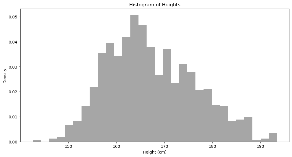
With this histogram, we can already do many things. For instance, we roughly know that if we randomly pick a person, the probability of this person having a height of 170 cm is less than having a height of 164 cm. But this estimation is very imprecise and requires visual inspection. In large-scale calculations, we cannot expect computers to look at this histogram every time they need to calculate the probability of a data point. What should we do?

We need a precise method to calculate the probability density at any arbitrary point (Evaluation Point).

First, height is a continuous variable, meaning height can be 1.71, 1.72, etc. So when comparing the probabilities of 170 and 164, we definitely cannot simply look at their respective frequencies.

A very simple solution is to consider points around 170 and 164, for example, comparing the densities of heights between 169-171 and 163-165. But one question remains: how wide should this “surrounding” range be?

This is a very classic problem. This range is called “bandwidth.”

There are many methods for selecting bandwidth. Let’s look at Scott’s rule:

$$h = \sigma \cdot n^{1/5}$$

Where $h$ is the calculated bandwidth, $\sigma$ is the standard deviation of all data, and $n$ is the number of data points. Note that $\sigma$ here treats all data as a population, not a sample, so Bessel’s correction is not needed.

sigma = np.std(heights)
n = len(heights)
h = sigma * n ** (-0.2)
print(f"Bandwidth: {h}")

Good, with this bandwidth, a very direct method is to compare the frequency of data points falling within $x \pm h$. $x$ is an evaluation point, such as 170 or 164.

x_170_freq = sum(170 - h <= height <= 170 + h for height in heights)
x_164_freq = sum(164 - h <= height <= 164 + h for height in heights)
print(f"The frequency of heights around 170cm is {x_170_freq}; the frequency around 164cm is {x_164_freq}")

Probability Density Function #

If we just want to compare which data point is more likely to appear in our data, our current method of comparing frequencies in their vicinity works. But often, we need to know the exact probability density of a given data point $x$ in our distribution. In other words, we want to know a specific probability density function (PDF): $\hat{f}_h (x)$.

I’ll give a few examples:

• You want to know which height is most likely to occur. You can use visual inspection and get approximately 164cm. You could also have the computer find the height with the highest frequency, but the problem is that the most likely height would necessarily be one that already exists in the data. If we have a specific PDF, we can find a point that may not necessarily exist in our data.
• Generating new samples: this is completely impossible with the frequency comparison method.
• Comparing model performance. A simple example: there are many ways to calculate bandwidth, but which one is best suited for our data? Each bandwidth choice corresponds to a different PDF. The simplest method is to provide a few new samples, calculate their probability densities, and determine which model maximizes the product of these densities. This indicates that the model maximizes the likelihood of new samples appearing. Of course, in actual calculations, we don’t compute the product but rather the sum of Log Likelihoods.

Now we understand the importance of deriving the probability density function $\hat{f}_h (x)$, but how do we obtain it? Mathematicians have long provided the answer:

$$\hat{f}_h (x) = \frac{1}{nh}\sum_{i=1}^n K\left( \frac{x - x_i}{h} \right) \tag{1}$$

Where:

• $n$ is the number of data points.
• $h$ is the bandwidth.
• $x$ is the point being evaluated (Evaluation Point).
• $x_i$ is one specific value from the existing data.
• $K$ is the kernel density function, which we’ll discuss below.

Before discussing the kernel density function, let’s first prove that:

$$\begin{aligned} \int_{-\infty}^\infty \hat{f}_h (x) dx & = \int \frac{1}{nh}\sum_{i=1}^n K\left( \frac{x - x_i}{h} \right)dx \\ & = \frac{1}{nh}\sum_{i=1}^n \int K\left( \frac{x - x_i}{h} \right)dx \\ & = \frac{1}{nh}\sum_{i=1}^n \int K(u)\cdot h \cdot du \\ & = \frac{1}{n}\sum_{i=1}^n \int K(u)\cdot du \\& = \frac{1}{n}\sum_{i=1}^n \\& = 1 \end{aligned}$$

Key points used here:

First, since $K$ is a kernel density function, necessarily $\int K(u)du = 1$.

For the variable substitution in the middle:

Let $u = \frac{x - x_i}{h}$, so we have $x = uh + x_i$, then take the derivative of $x$ with respect to $u$ (how does $x$ change when $u$ increases slightly):

$$\frac{dx}{du} = \frac{d}{du}(hu + x_i) = h \Rightarrow dx = h \cdot du$$

Gaussian Kernel #

The Gaussian kernel is a very commonly used kernel density function in KDE.

Let’s recall that the probability density function of a Gaussian distribution is:

$$f(x) = \frac{1}{\sqrt{2\pi \sigma^2}}e^{-\frac{1}{2} \left(\frac{x - \mu}{\sigma}\right)^2}$$

Let $$u = \frac{x - x_i}{h}$$

The commonly used kernel density function is:

$$K(u) = \frac{1}{\sqrt{2 \pi}}e^{- \frac{u^2}{2}}$$

Comparing, you’ll see this is the PDF of $\mathcal{N}(0,1)$.

Most statistics textbooks don’t go into this much detail. But even at this point, the curious among you might still wonder: while the substitution $u = \frac{x - x_i}{h}$ makes the expression look cleaner, we suddenly lose sight of how the entire probability density function $\hat{f}_h (x)$ relates to $x$.

Let’s express it in terms of $x$:

$$K_h(x) = \frac{1}{\sqrt{2\pi}} e^{-\frac{1}{2} \left( \frac{x - x_i}{h} \right)^2}$$

Comparing with the standard normal distribution density function, we notice that if we change $\sqrt{2\pi}$ to $\sqrt{2\pi h^2}$, then $K_h(x)$ would be the probability density function of $\mathcal{N}(x_i, h^2)$. But the problem is, $h^2$ doesn’t appear in the formula!

Actually, going back to formula (1), if we remove $\frac{1}{h}$:

$$\hat{f}_h (x) = \frac{1}{n}\sum_{i=1}^n K_i(x)$$

And then set the kernel density function as:

$$K_i(x) = \frac{1}{\sqrt{2\pi h^2}} e^{-\frac{1}{2} \left( \frac{x - x_i}{h} \right)^2}$$

Everything makes sense, and it’s more intuitive.

How to understand this: For any new data point $x$, we want to calculate its probability density. How? We find each point $x_i$ in the original data (heights), and calculate the probability density of $x$ in $\mathcal{N}(x_i, h^2)$. Then we sum all these probability densities, and that’s the probability density of the new data point $x$ in this unknown distribution.

Summary #

To summarize, formula (1) can be written as:

$$\hat{f}_h (x) = \frac{1}{nh}\sum_{i=1}^n K(u) \tag{1}$$

Where:

• $u = \frac{x - x_i}{h}$.
• $K(u) = \frac{1}{\sqrt{2 \pi}}e^{- \frac{u^2}{2}}$, representing the probability density function of $\mathcal{N}(0,1)$.

Formula (1) can also be written as:

$$\hat{f}_h (x) = \frac{1}{n}\sum_{i=1}^n K_i(x) \tag{2}$$

Where: $$K_i(x) = \frac{1}{\sqrt{2\pi h^2}} e^{-\frac{1}{2} \left( \frac{x - x_i}{h} \right)^2}$$

Representing the probability density function of $\mathcal{N}(x_i, h^2)$.

Both expressions are valid. People tend to prefer the first one because it explicitly shows that $h$ is constant. In the second formula, $h$ is hidden within $K_i(x)$, which is less obvious.

Calculation #

Next, let’s do a concrete calculation.

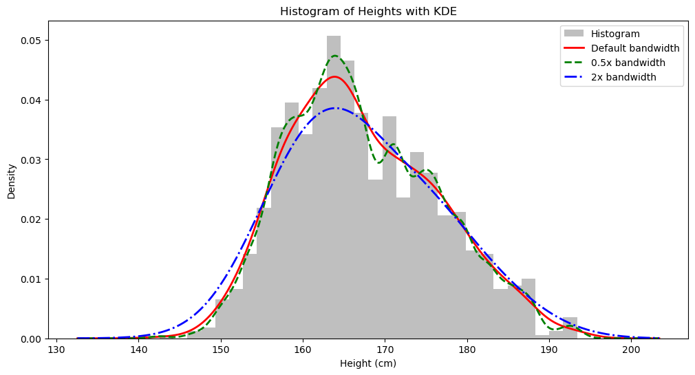
Another very useful aspect of KDE is visualization: we can plot the possible underlying distribution continuously rather than just using a histogram.

How do we plot it? Since $\hat{f}_h (x)$ can give us the specific probability density of a data point $x$ in the distribution, we can find 1000 points from the lowest to the highest height in our distribution, calculate the probability density for each point, connect them, and that’s our KDE curve.

min(heights), max(heights)

import math 
from numba import njit 

SQRT_2PI = math.sqrt(2.0 * math.pi)

@njit(fastmath=True)
def gaussian_kernel(x: float, xi: float, bw: float) -> float:
    """ calculate K_i(x)
    """
    z = (x - xi) / bw
    return math.exp(-0.5 * z * z) / (bw * SQRT_2PI)

@njit(fastmath=True)
def calculate_bandwidth(data: np.ndarray, scale:float=1.0) -> float:
    n = len(data)
    sigma = max(np.std(data), 1e-12)
    return sigma * n ** (-0.2) * scale

@njit(fastmath=True)
def _compute_pdf(x: float, data: np.ndarray, bw: float) -> float:
    """Compute PDF of an evaluation point (x)
    """
    pdf = 0.0 
    for j in range(len(data)):
        pdf += gaussian_kernel(x, data[j], bw)
    return pdf/len(data)

def obtain_densities(xs: np.ndarray, data: np.ndarray, bw_scale: float = 1.0) -> np.ndarray:
    densities = np.zeros(len(xs))
    bw = calculate_bandwidth(data, scale = bw_scale)
    for idx, x in enumerate(xs):
        densities[idx] = _compute_pdf(x, data, bw)
    return densities 

# Create evaluation points for KDE
x_min = min(heights) - 10
x_max = max(heights) + 10
x_eval = np.linspace(x_min, x_max, 1000)

# Compute KDE
densities = obtain_densities(x_eval, heights)
densities_half_bw_scale = obtain_densities(x_eval, heights, bw_scale = 0.5)
densities_double_bw_scale = obtain_densities(x_eval, heights, bw_scale = 2)

# Create the plot
plt.figure(figsize=(12, 6))

# Plot histogram
plt.hist(heights, bins=30, density=True, alpha=0.5, color='gray', label='Histogram')

# Plot KDE
plt.plot(x_eval, densities, 'r-', linewidth=2, label='Default bandwidth')

plt.plot(x_eval, densities_half_bw_scale, 'g--', linewidth=2, label='0.5x bandwidth')

plt.plot(x_eval, densities_double_bw_scale, 'b-.', linewidth=2, label='2x bandwidth')

# Add labels and legend
plt.title('Histogram of Heights with KDE')
plt.xlabel("Height (cm)")
plt.ylabel("Density")
plt.legend()

# Optional: show statistics
bw = calculate_bandwidth(heights)
print(f"Bandwidth used: {bw:.2f}")
print(f"Number of data points: {len(heights)}")
print(f"Mean height: {np.mean(heights):.2f} cm")
print(f"Standard deviation: {np.std(heights):.2f} cm")

# Show plot
plt.show()

Let’s calculate and visualize using Scipy:

# Optional: Compare bandwidths
# Calculate the bandwidth that scipy uses
bw_scipy = kde.factor * np.std(heights) * (len(heights) ** (-1/5))
# print(f"Scipy bandwidth: {bw_scipy:.2f}")

# Explicitly compare different bandwidths (optional)
plt.figure(figsize=(12, 6))
plt.hist(heights, bins=30, density=True, alpha=0.5, color='gray', label='Histogram')

# Default bandwidth
kde1 = stats.gaussian_kde(heights)
plt.plot(x_eval, kde1(x_eval), 'r-', linewidth=2, label='Default bandwidth')

# Custom bandwidth (0.5x default)
kde2 = stats.gaussian_kde(heights, bw_method=kde.factor * 0.5)
plt.plot(x_eval, kde2(x_eval), 'g--', linewidth=2, label='0.5x bandwidth')

# Custom bandwidth (2x default)
kde3 = stats.gaussian_kde(heights, bw_method=kde.factor * 2)
plt.plot(x_eval, kde3(x_eval), 'b-.', linewidth=2, label='2x bandwidth')

plt.title('Effect of Different Bandwidths on KDE Using Scipy')
plt.xlabel('Height (cm)')
plt.ylabel('Density')
plt.legend()
plt.show()

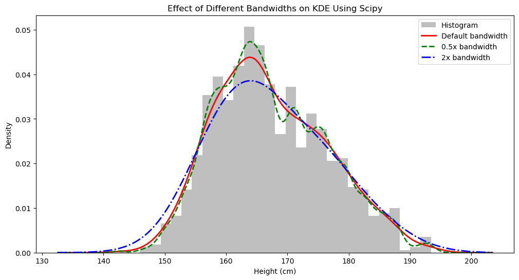
We can see that our self-defined method is correct because the results are the same.

Weighted KDE #

Sometimes, each data point in the original data has a corresponding weight. For example, a height of 170 cm has an 80% probability of belonging to a male and a 20% probability of belonging to a female. With weights, both the bandwidth and $\hat{f}_h (x)$ calculation methods change accordingly.

With weights, Scott’s bandwidth calculation method becomes:

$$h = \sigma_w \cdot n_\text{eff}^{-1/5}$$

If each data point $x_i$ has a corresponding weight $w_i$, we have:

$$\mu_w = \frac{\sum w_i x_i}{\sum w_i}$$

$$\sigma_w^2 = \frac{\sum w_i (x_i - \mu_w)^2}{\sum w_i}$$

$$n_\text{eff} = \frac{1}{\sum w_i^2}$$

Correspondingly, the probability density function becomes:

$$\hat{f}_h (x) = \sum_{i=1}^n w_i \frac{1}{\sqrt{2\pi h^2}} e^{-\frac{1}{2} \left( \frac{x - x_i}{h} \right)^2} \tag{3}$$

Note that $w$ must be normalized, i.e., $\sum_{i=1}^n w_i = 1$. If uncertain, a more rigorous expression for the weighted KDE probability density function is:

$$\hat{f}_h (x) = \frac{\sum_{i=1}^n w_i \frac{1}{\sqrt{2\pi h^2}} e^{-\frac{1}{2} \left( \frac{x - x_i}{h} \right)^2}}{\sum_{i=1}^n w_i} \tag{3}$$

Last modified on 2025-04-17