Least squares #
Matrix equations: $Ax = b$
If you have more equations than variables, i.e., when $A$ is tall (overdetermined), for example
$$ A = \begin{bmatrix} 2 & 3 \\ 4 & -1 \\ 2 & 1 \end{bmatrix} $$
And
$$ x = \begin{bmatrix} x_1 \\ x_2 \end{bmatrix} $$
$$ b = \begin{bmatrix} 1 \\ 2 \\ 3 \end{bmatrix} $$
More often than not, you don’t have viable solutions. One fix is to use least squares.
If you have more variables than equations (e.g., you only have $2x + 3y = 0$), i.e., when $A$ is wide:
$$ A = \begin{bmatrix} 2 & 3 \end{bmatrix} $$
And
$$ x = \begin{bmatrix} x_1 \\ x_2 \end{bmatrix} $$
$$ b = 0 $$
it means you either have no solutions or have infinitely many solutions. One solution is to use regularization.
Least squres: to minimize $||Ax - b||^2$ and subject to $x$.
Interpretation #
The graphcal interpretation of minimizing $||Ax - b||^2$
Take the above example as an instance.
$$ A = \begin{bmatrix} 2 & 3 \\ 4 & -1 \\ 2 & 1 \end{bmatrix} $$
$$ x = \begin{bmatrix} x_1 \\ x_2 \end{bmatrix} $$
$$ \vec{b} = \begin{bmatrix} 1 \\ 2 \\ 3 \end{bmatrix} $$
We write
$$ a_1 = \begin{bmatrix} 2 \\ 4 \\ 2 \end{bmatrix} $$
and
$$ a_2 = \begin{bmatrix} 3 \\ -1 \\ 1 \end{bmatrix} $$
So we are actually minimizing
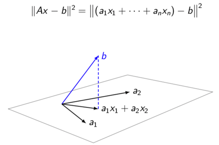
$$||\vec{a_1}x_1 + \vec{a_2}x_2 - \vec{b}||^2$$
It should be noted that $\vec{a_1}x_1 + \vec{a_2}x_2$ is a vector itself (Let’s denoted it as $\vec{t}$) and it is on the plane defined by $\vec{a_1}$ and $\vec{a_2}$. So the above objective is to minimize the length of the vector $\vec{t} - \vec{b}$. This is equivalent to finding the projection of $\vec{b}$ on the plane defined by $\vec{a_1}$ and $\vec{a_2}$.
Also note that if the equations have a solution, for example
$$ A = \begin{bmatrix} 2 & 1 \\ 3 & -1 \end{bmatrix} $$
$$ x = \begin{bmatrix} x_1 \\ x_2 \end{bmatrix} $$
$$ \vec{b} = \begin{bmatrix} 1 \\ 2 \end{bmatrix} $$
So
$$ a_1 = \begin{bmatrix} 2 \\ 3 \end{bmatrix} $$
and
$$ a_2 = \begin{bmatrix} 5 \\ 7 \end{bmatrix} $$
We have
$$ \vec{a_1}x_1 + \vec{a_2}x_2 = \vec{b} $$
In this case, $\vec{b}$ is on the plane defined by $\vec{a_1}$ and $\vec{a_2}$.
In the case previously, because there are no solutions, $\vec{b}$ is not on the plane defined by $\vec{a_1}$ and $\vec{a_2}$. What we want to do is to find a vector on the plane defined by $\vec{a_1}$ and $\vec{a_2}$ that is as close to $\vec{b}$ as possible.
Norm #
- One norm:
$||r||_1 = |r_1| + |r_2| + ... |r_n|$ - Two norm (aka Euclidean distance):
$||r||_2 = \sqrt{{r_1}^2 + {r_2}^2 + ... + {r_n}^2}$
Curve Fitting (Regression) #
Suppose we are giving two series of numbers:
x = [ 1, 2, 3, 4, 5, 6, 7, 8, 9, 10, 11, 12, 13, 14, 15, 16 ]
y = [ 1, 3, 0, 1, 2, 4, 6, 7, 5, 5, 6, 7.2, 5.5,  4, 3.2, 5]
And we suspect that they are related by a fourth-degree polynomial $y = u_1x^4 + u_2x^3 + u_3x^2 + u_4x + u_5$. How can we find all the $u$s that best agree with our data? Using least squares!
using Plots, Gurobi, JuMP, Polynomialsx = [ 1, 2, 3, 4, 5, 6, 7, 8, 9, 10, 11, 12, 13, 14, 15, 16 ]
y = [ 1, 3, 0, 1, 2, 4, 6, 7, 5, 5, 6, 7.2, 5.5, 4, 3.2, 5]
Plots.scatter(x, y,
label="",
xlabel="x",
ylabel="y"
)
savefig("/en/blog/2023-03-22-least-square_files/least-squares-01.png")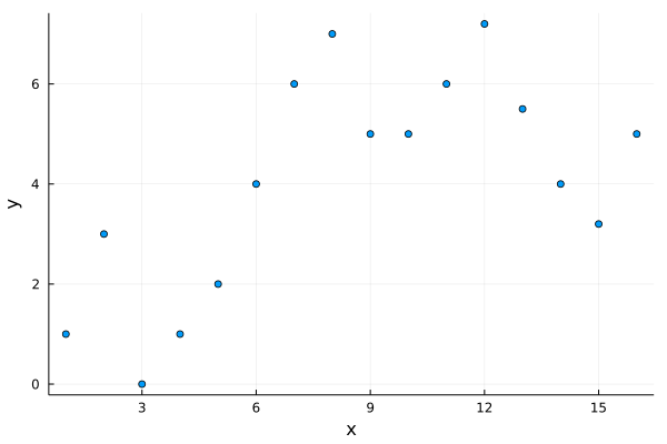
k = 4
n = length(x)
A = zeros(n, k+1)

# get the A matrix
for i in 1:n
    A[i,:] = [x[i]^m for m in k:-1:0]
end
Something like this but with a higher degree:
m = Model(Gurobi.Optimizer)

@variable(m, u[1:k+1])
@objective(m, Min, sum( (y - A*u).^2 ))

optimize!(m)u = value.(u)A simpler way #
In fact, there is a much simpler way. Because the above operations are used frequently, there is a special operator for that: \
u = A\yPlots.scatter(x, y,
label="",
xlabel="x",
ylabel="y"
)
f(x) = u[1]*x^4 + u[2]*x^3 + u[3]*x^2 + u[4]*x + u[5]
# use continuous x range; otherwise the fit line is discrete
xs = 1:0.01:16
Plots.plot!(xs, f,
linecolor = "green",
linewidth = 2,
label = "fourth-degree polynomial fit line"
)
savefig("/en/blog/2023-03-22-least-square_files/least-squares-02.png")
When polynomials have much higher orders, it is best to use the Polynomials package rather than writting it manually like f(x) = u[1]*x^4 + u[2]*x^3 + u[3]*x^2 + u[4]*x + u[5]. In Polynomials, the power order increases, i.e., f(x) = u[1]x + u[2]x^2 + u[3]x^3 ..., so we need to reverse the order of u:
p = Polynomial(reverse(u))4.3206730769230814 - 3.3515882584477747∙x + 0.9697320046439619∙x2 - 0.08461679037336926∙x3 + 0.002320865086925458∙x4
ys = p.(xs)
Plots.scatter(x, y,
    label="",
    xlabel="x",
    ylabel="y"
)

# note it is is (xs, ys) rather than (xs, p)
Plots.plot!(xs, ys,
    linecolor = "green",
    linewidth = 2,
    label = "fourth-degree polynomial fit line"
)

savefig("/en/blog/2023-03-22-least-square_files/least-squares-03.png")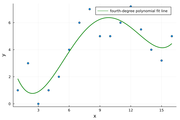
Last modified on 2025-07-02 • Suggest an edit of this page