TopBrass Revisited #
Back to the TopBrass problem:
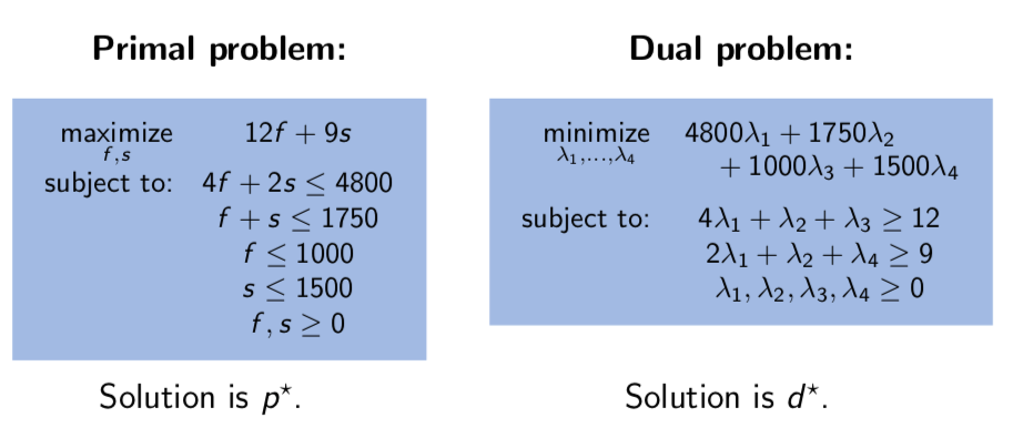
Top Brass Trophy Company makes large championship trophies for youth athletic leagues. At the moment, they are planning production for fall sports: football and soccer. Each football trophy has a wood base, an engraved plaque, a large brass football on top, and returns 12 USD in profit.
Soccer trophies are similar except that a brass soccer ball is on top, and the unit profit is 9 USD.
Since the football has an asymmetric shape, its base requires 4 board feet of wood; the soccer base requires only 2 board feet.
There are 1000 brass footballs in stock, 1500 soccer balls, 1750 plaques, and 4800 board feet of wood. What trophies should be produced from these supplies to maximize total profit assuming that all that are made can be sold?
This translates into the following optimization problem:
Max 12 f + 9 s
Subject to
 4 f + 2 s ≤ 4800.0
 f + s ≤ 1750.0
 f ≥ 0.0
 s ≥ 0.0
 f ≤ 1000.0
 s ≤ 1500.0
What we want to do is to find the upper bound of $12f + 9s$. Given that $f \le 1000$ and $s \le 1500$, we know that
$$12f + 9s \le 12\cdot 1000 + 9\cdot 1500 = 25500$$
But this is not the best upper bound. We can improve it:
$$12f + 9s \le f + (4f + 2s) + 7 \cdot (f + s) \le 1000 + 4800 + 1750 \cdot 7 = 18050$$
Again, it is not the best upper bound, and we can keep improving it. From $f + s ≤ 1750$, we know
$$12f + 9s \le 12f + 12s \le 1750\times 9 = 15750$$
Is this the optimal upper bound? Definitly not. But you get the idea that if we have $\lambda_1$, $\lambda_2$, $\lambda_3$, $\lambda_4 \ge 0$, then by choosing the best possible values of them, we can have the optimal upper bound for $12f + 9s$:
$$12f + 9s \le \lambda_1(4f + 2s) + \lambda_2 (f + s) + \lambda_3 f + \lambda_4 s$$
Based on the constraints we have, we know:
$$12f + 9s \le 4800\lambda_1 + 1750 \lambda_2 + 1000 \lambda_3 + 1500 \lambda_4$$
What we want is the lower bound of $4800\lambda_1 + 1750 \lambda_2 + 1000 \lambda_3 + 1500 \lambda_4$, i.e., we want to minimize it.
Then, what are the new contraints?
Based on
$$12f + 9s \le \lambda_1(4f + 2s) + \lambda_2 (f + s) + \lambda_3 f + \lambda_4 s$$
we know
$$0 \le (4\lambda_1 + \lambda_2 + \lambda_3 - 12)f + (2\lambda_1 + \lambda_2 + \lambda_4 - 9)s$$
We also know that both $f$ and $s$ are larger than or equal to $0$, but we do not know which one ($f$ or $s$) is larger. Therefore, to make sure $0 \le (4\lambda_1 + \lambda_2 + \lambda_3 - 12)f + (2\lambda_1 + \lambda_2 + \lambda_4 - 9)s$, we can ensure that
$$4\lambda_1 + \lambda_2 + \lambda_3 - 12 \ge 0$$
and
$$2\lambda_1 + \lambda_2 + \lambda_4 - 9 \ge 0$$
Therefore, the original optimization problem is converted to:
Minimize $4800\lambda_1 + 1750 \lambda_2 + 1000 \lambda_3 + 1500 \lambda_4$
Subject to:
$4\lambda_1 + \lambda_2 + \lambda_3 \ge 12$$2\lambda_1 + \lambda_2 + \lambda_4 \ge 9$$\lambda_1$,$\lambda_2$,$\lambda_3$,$\lambda_4 \ge 0$
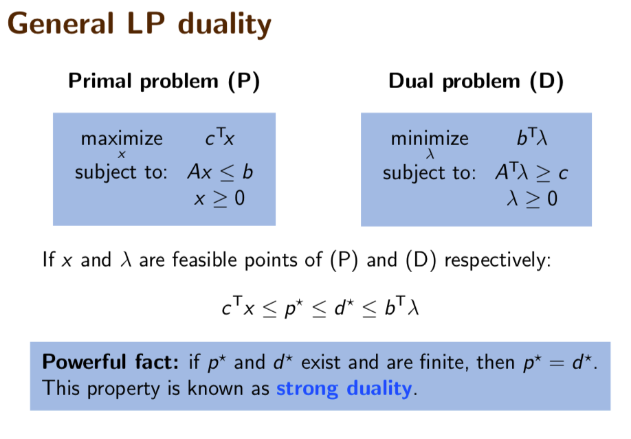
Using matrix: #
Primal problem #
$$ \begin{align*} \underset{f,s}{\text{maximize}}\qquad& \begin{bmatrix} 12 \\ 9 \end{bmatrix}^{T} \begin{bmatrix} f \\ s \end{bmatrix}\\ \text{subject to:}\qquad& \begin{bmatrix} 4 & 2 \\ 1 & 1 \\ 1 & 0 \\ 0 & 1 \end{bmatrix} \begin{bmatrix} f \\ s \end{bmatrix} \le \begin{bmatrix} 4800 \\ 1750 \\ 1000 \\ 1500 \end{bmatrix}\\ & f, s \ge 0 \end{align*} $$
Dual problem #
$$ \begin{align*} \underset{\lambda_1, \lambda_2, \lambda_3, \lambda_4}{\text{minimize}}\qquad& \begin{bmatrix} 4800 \\ 1750 \\ 1000 \\ 1500 \end{bmatrix}^{T} \begin{bmatrix} \lambda_1 \\ \lambda_2 \\ \lambda_3 \\ \lambda_4 \end{bmatrix}\\ \text{subject to:}\qquad& \begin{bmatrix} 4 & 1 & 1 & 0 \\ 2 & 1 & 0 & 1 \end{bmatrix} \begin{bmatrix} \lambda_1 \\ \lambda_2 \\ \lambda_3 \\ \lambda_4 \end{bmatrix} \ge \begin{bmatrix} 12 \\ 9 \end{bmatrix}\\ & \lambda_1, \lambda_2, \lambda_3, \lambda_4 \ge 0 \end{align*} $$
General form: #
Implementation #
Primal problem #
using HiGHS, JuMP

m = Model(HiGHS.Optimizer)

@variable(m, 0<= f <= 1000)
@variable(m, 0<= s <= 1500)
@objective(m, Max, 12*f + 9*s)
@constraint(m, 4*f + 2*s <= 4800) # board feet of wood
@constraint(m, f + s <= 1750)

optimize!(m)

println("--------------------------------------------")

println("The total number of football trophies is ", Int(value(f)))
println("The total number of soccer trophies is ", Int(value(s)))
println("The highest possible profit is \`$", objective_value(m))
Running HiGHS 1.4.2 [date: 1970-01-01, git hash: f797c1ab6]
Copyright (c) 2022 ERGO-Code under MIT licence terms
Presolving model
2 rows, 2 cols, 4 nonzeros
2 rows, 2 cols, 4 nonzeros
Presolve : Reductions: rows 2(-0); columns 2(-0); elements 4(-0) - Not reduced
Problem not reduced by presolve: solving the LP
Using EKK dual simplex solver - serial
  Iteration        Objective     Infeasibilities num(sum)
          0     0.0000000000e+00 Ph1: 0(0) 0s
          2     1.7700000000e+04 Pr: 0(0) 0s
Model   status      : Optimal
Simplex   iterations: 2
Objective value     :  1.7700000000e+04
HiGHS run time      :          0.00
--------------------------------------------
The total number of football trophies is 650
The total number of soccer trophies is 1100
The highest possible profit is $`17700.0
Dual problem #
m = Model(HiGHS.Optimizer)
vectorB = [4800, 1750, 1000, 1500]
vectorA = [4 2 ; 1 1; 1 0; 0 1]
vectorC = [12, 9]

@variable(m, λ[1:4] >= 0)
@objective(m, Min, vectorB'*λ)
@constraint(m, vectorA'*λ .>= vectorC)
optimize!(m)

println("--------------------------------------------")
println("Obective \`$", objective_value(m))
println("λ: ", value.(λ))
Running HiGHS 1.4.2 [date: 1970-01-01, git hash: f797c1ab6]
Copyright (c) 2022 ERGO-Code under MIT licence terms
Presolving model
2 rows, 4 cols, 6 nonzeros
2 rows, 4 cols, 6 nonzeros
Presolve : Reductions: rows 2(-0); columns 4(-0); elements 6(-0) - Not reduced
Problem not reduced by presolve: solving the LP
Using EKK dual simplex solver - serial
  Iteration        Objective     Infeasibilities num(sum)
          0     0.0000000000e+00 Pr: 2(21) 0s
          3     1.7700000000e+04 Pr: 0(0) 0s
Model   status      : Optimal
Simplex   iterations: 3
Objective value     :  1.7700000000e+04
HiGHS run time      :          0.00
--------------------------------------------
Obective $`17700.0
λ: [1.5, 6.0, 0.0, 0.0]
Sensitivity #
The dual has practical meanings. First, in our above example, the two problems have strong duality. That is to say, the maximum of $12f + 9s$ is equal to the minimum of $4800\lambda_1 + 1750 \lambda_2 + 1000 \lambda_3 + 1500 \lambda_4$.
Both can be regarded as the total profits. Then, what $\lambda_1$ mean here? Since the units is USD, and we have 4800 board feet of wood, $\lambda_1$ here indicates the price that wood is worth. It is called shadow price.
Through the results of the dual problem, we know $\lambda_1 = 1.5$. That means that each board feet of wood is worth 1.5 USD.
What if someone now is selling wood at 1 dollar per board feet. Is that a good offer? Of course! You see, if we buy 400 feet of wood at that price, which cose 400 Dollars. What will be the increase in the profits?
Because the solution to the primal is the same as that to the dual, then we know the total profits are still
$$4800\lambda_1 + 1750 \lambda_2 + 1000 \lambda_3 + 1500 \lambda_4$$
But since we have 400 more feet of wood, the profits would be
$(4800 + 400)\lambda_1 + 1750 \lambda_2 + 1000 \lambda_3 + 1500 \lambda_4$
And because $\lambda_1 = 1.5$, so the profits will go up by 600! It’s a good deal, isn’t it?
Complementary Slackness #
In the solution to the dual problem, we noticed that
λ: [1.5, 6.0, 0.0, 0.0]
We say that the contraints for wood and plague are becoming tight because $\lambda_1$ and $\lambda_2$ are non-zero. We say that the contraints for brass football and soccer ball have slack, because $\lambda_3$ and $\lambda_4$ are zero.
Last modified on 2023-03-17