Notes on 3blue1brown Essence of Calculus

Lesson 1: Preview #

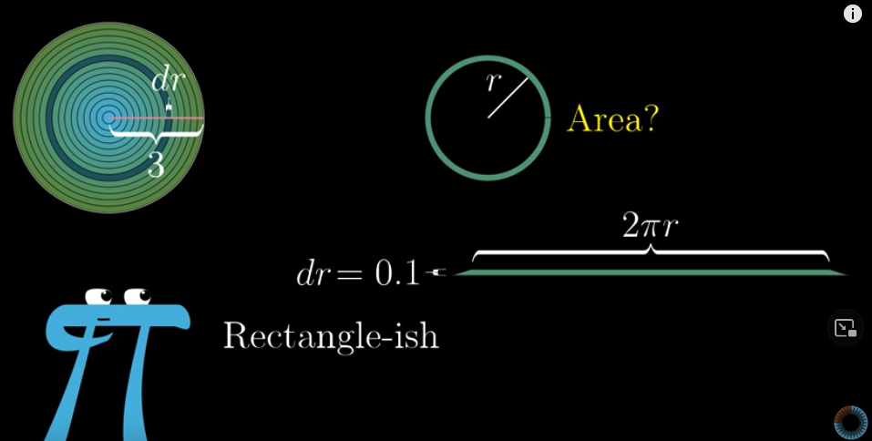
Think about the area of a circile. We know that it’s area is $\pi R^2$. But, why?

We can solve the problem this way. Imagine that we divide a radius of this circle into many smaller pieces, each with a width of $dr$. Then this circle will be composed of many rings. If we tear a ring open and flatten it, it will become a rectangle-ish shape. The length of this “rectangle” is the circumference of this ring and the width is $dr$. The area of this ring is the area of this “rectangle”. If we denote the radius of this ring as $r$, its circumference will be $2\pi r$, so the area of it is $2\pi r \cdot dr$.

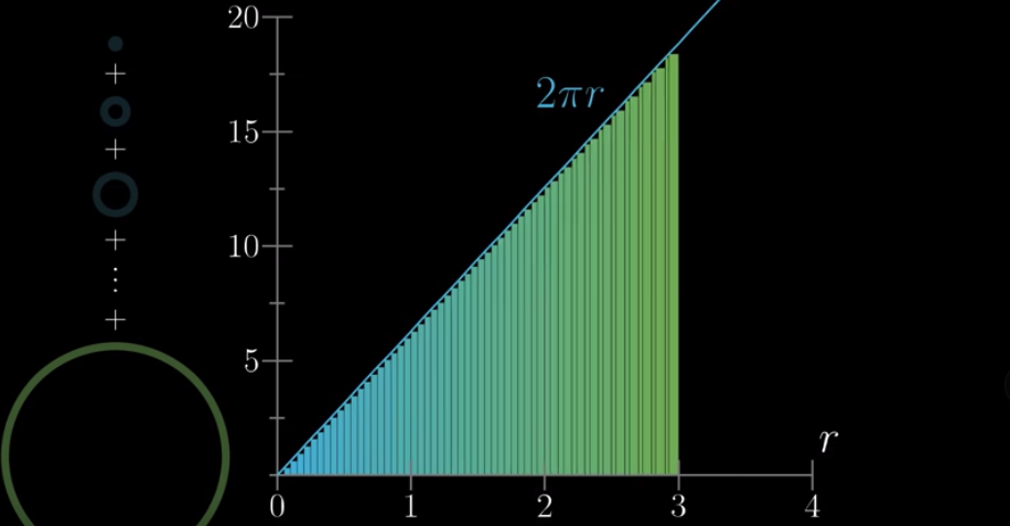
You can also image stacking every ring vertically, sorted by their length. When $dr$ is small enough, the area of all these vertically stacked rings will be a triangle, and the area of the circle can be approximated by the area of this triangle. The base of this triangle is the radius of the circle, $R$, and the hight of this triangle is the length of the biggest ring, which is $2\pi R$. Therefore, the area of this triangle, or this circle, is $\frac{2\pi R \cdot R}{2} = \pi R^2$.

Moving further #

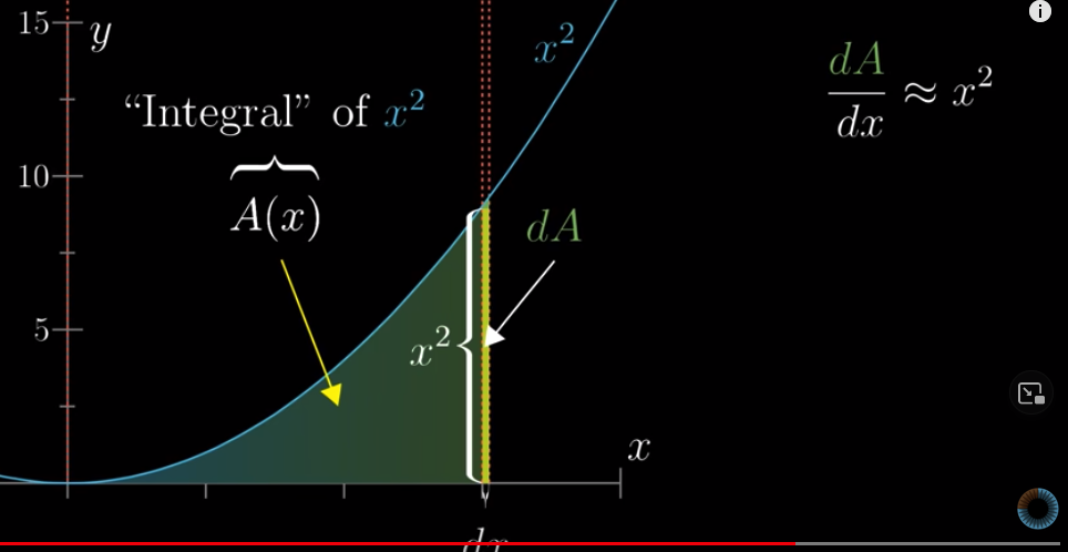
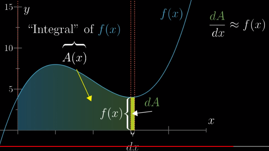
What if we want to know the area of the graph of this function: $y = x^2$?

Let’s define a function: the area of the graph between $x=0$ and $x$ is $A(x)$. With this function, we want to know what the area is at any $x$ value. We call this $A(x)$ as the “integral” of $x^2$. It’s a difficult problem to know what $A(x)$ is but we know it should have this property. If we increase $x$ a little bit, say, by $dx$, the increase in area, which we denote as $dA$, can be approximated by the rectangle whose area is $x^2 dx$. By the way, $dx$ means “difference in $x$” and $dA$ means difference in Area. Since $dA \approx x^2 dx$, we have:

$$\frac{dA}{dx} \approx x^2$$

A concrete example:

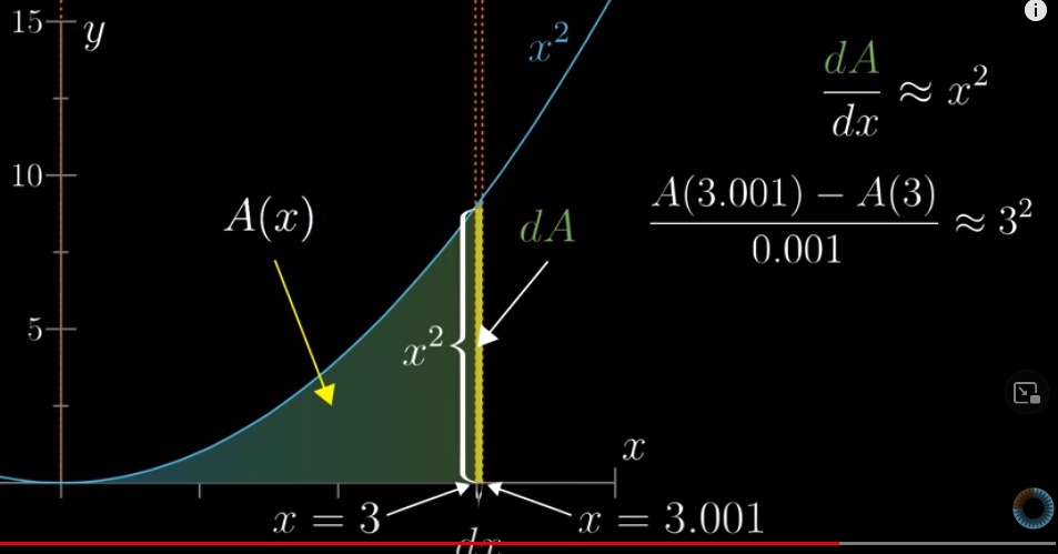
In fact, the graph can be one of any functions and what we discussed above remains true. For example,

Lesson 2: The paradox of the derivative #

Derivative can been seen as the approximation of the rate of change.

Let’s say a car is moving. We plot how much distance the car moves against time. That is to say, we plot this function: $Distance = f(Time)$. Note that we use the cumulative distance.

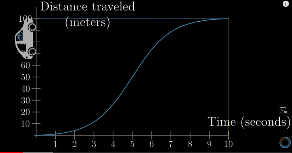
For example, the distance when $t=2$ tells us the total distance the car has travelled after 2 seconds. Let’s denote the distance as $s(t)$.

We can also plot the speed, or velocity, of this car against time as well:

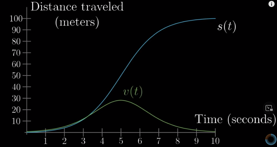
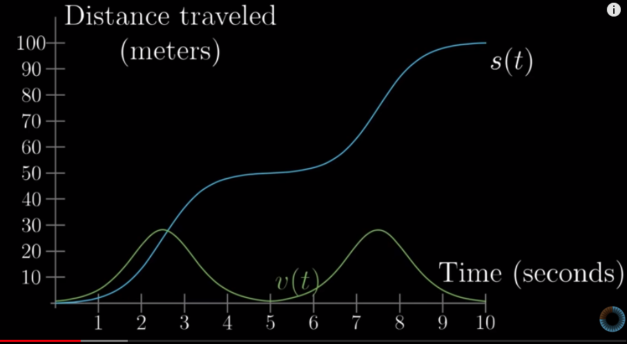
The velocity curve is definitly related to the $s(t)$ curve:

Now, a question is: what does velocity really mean? Say, we can know the velocity at $t=3$. But how can you tell the speed of a car at a single moment? Suppose you saw a picture of car moving without any referencing point, how can you know the speed of it?

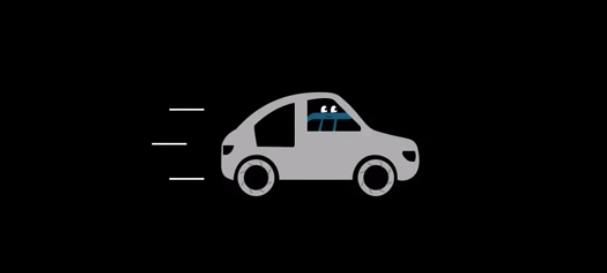
No, you cannot. The speed is about change, so we need to compare two time points.

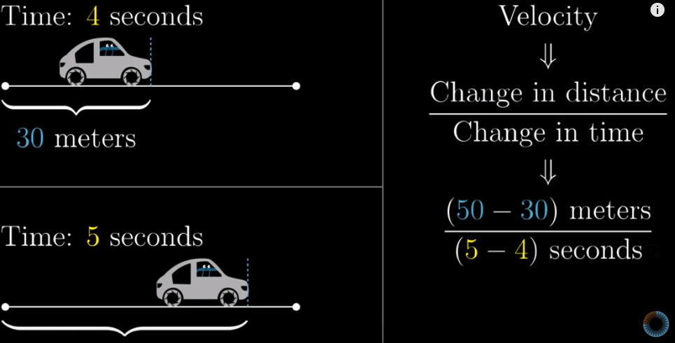
In fact, this is how car companies calculate the speed: they look at the distance travelled after a tiny amount of time. For example, we can look at how much distance is travelled between $t=3$ and $t=3.01$. We devide that change in distance by the change in time, then we get the velocity, or speed.

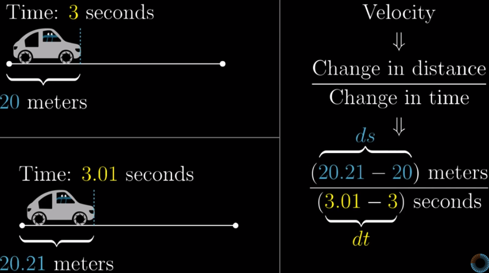
Okay, let’s go back to our question: what does velocity at $t = 3$ mean? It means the distance between $t=3$ and a tiny amount of time after that, say, $t=3.01$.

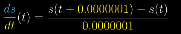
When we calculate the speed, we use this: $\frac{ds}{dt}$. This is almost derivative, but not quite yet. The real derivative is that which you are approaching when $t$ is approaching $0$:

Then, what is this ratio, i.e., $\frac{ds}{dt}$, approaching? Let’s take a look.

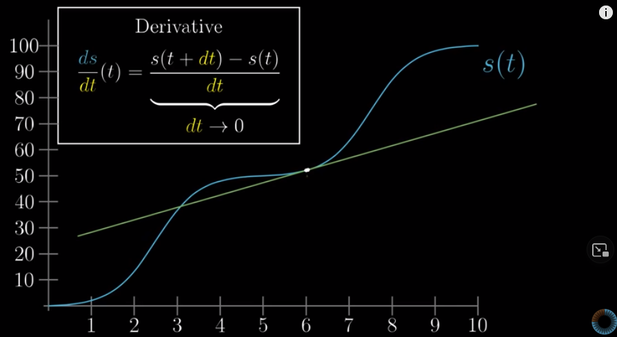
The change in distance over change in time is the slope of line connecting the two points we are comparing:

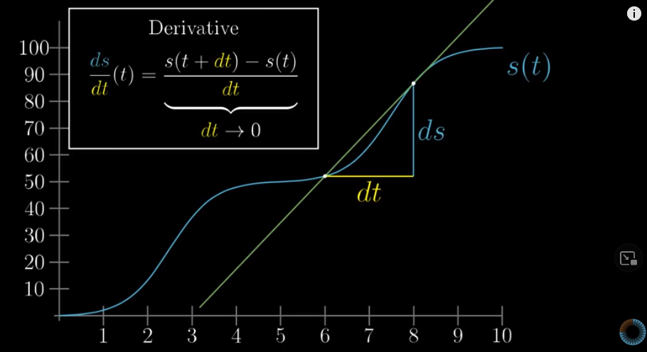
When $dt$ approaches zero, the two points get closer and closer and the line is almost the line that is tangent to the graph at the point $t$ we are looking at.

However, $t$ is only approaching zero, but never will be zero. So we should interpret the velocity at $t$ as the best approximation of its speed at that time point.

Let’s compute for a concrete example.

Let’s say the function of time and distance is this: $s(t) = t^3$. And we look at $t=2$. This will be it’s speed:

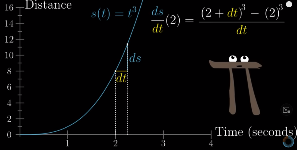
When you calculate it, the result will be:

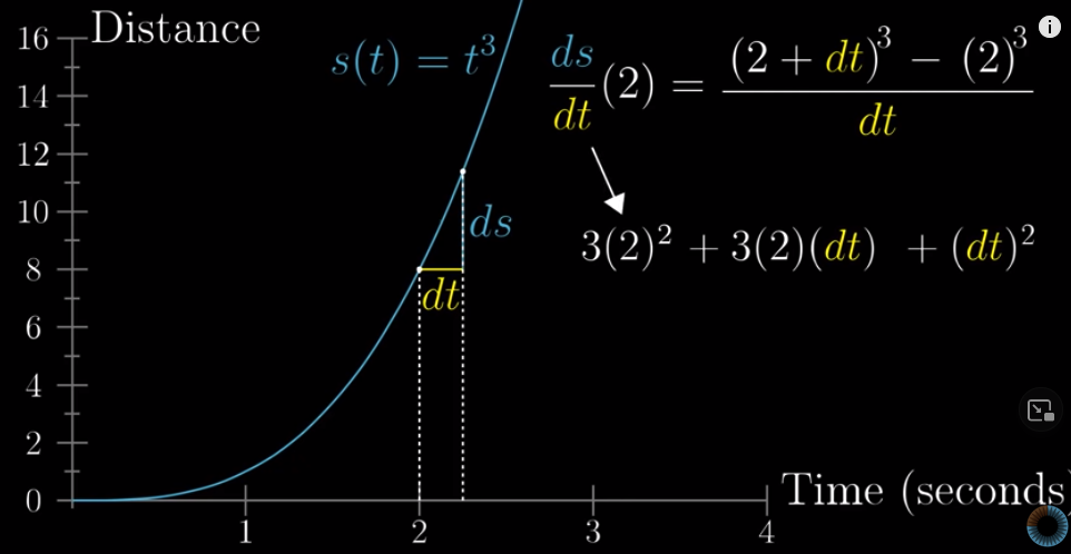
As $dt$ approaches zero, we can ignore the last two terms and the speed at any $t$ is approximately $3\cdot2^2$.

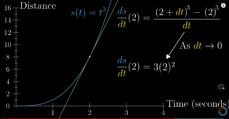
This applies to any time point. That is to say, if the function of time and distance is $s(t) = t^3$, the speed at any time can be approximated as $3t^2$.

Wait, what about $t=0$ ? The speed is zero. But does that mean that the car i s not moving at $t=0$?

No. What it says is that when we compare two time moments, $t=0$ and $t=0+dt$, when $dt$ is approaching zero, the change in distance over the change in time, is also approaching zero.

We can use the calculation above to know why.

$$\frac{ds}{dt} (0) = 3\cdot0^2 + 3\cdot0\cdot dt + (dt)^2 = (dt)^2$$

So, as $dt$ approaches zero, the speed at $t=0$ also approaches zero.

So the speed of 0 is only an approximation.

Lesson 3: Derivative fomulas through geometry #

“Tiny nudges are the heart of derivatives.”

How to compute the derivative of a given function?

Let’s take a concrete example: $f(x) = x^2$. Let’s denote the tiny change in $x$ as $dx$ and the resulting change in $f(x)$ as $df$.

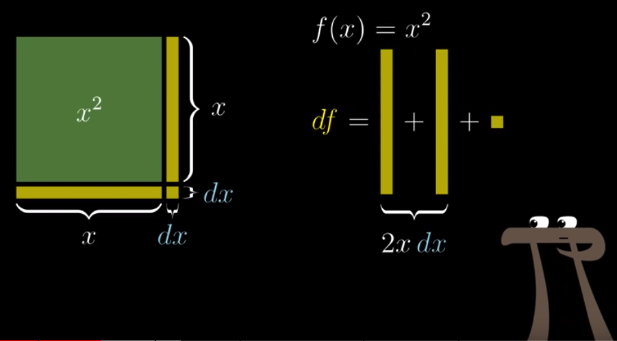
So we have: $df = 2x\cdot dx + (dx)^2$. Then we devide it by $dx$ and we have:

$$\frac{df}{dx}= 2x + {dx}$$

Because $dx$ is approaching zero, we can safely ignore $dx$ and say that the derivative of $f(x)=2x$ is $2x$.

The same is for $f(x) = x^3$.

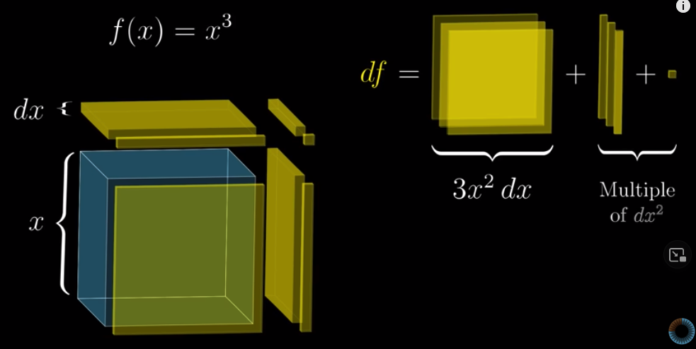
We have: $df = 3x^2\cdot dx + 3x\cdot(dx)^2 + (dx)^3$. Then we devide the whole thing by $dx$ and we have:

$$\frac{df}{dx} = 3x^2 + 3x\cdot dx + {dx}^2$$ Again, we can safely ignore $3x\cdot dx + {dx}^2$ and say that the derivative of $f(x)=x^3$ is $3x^2$.

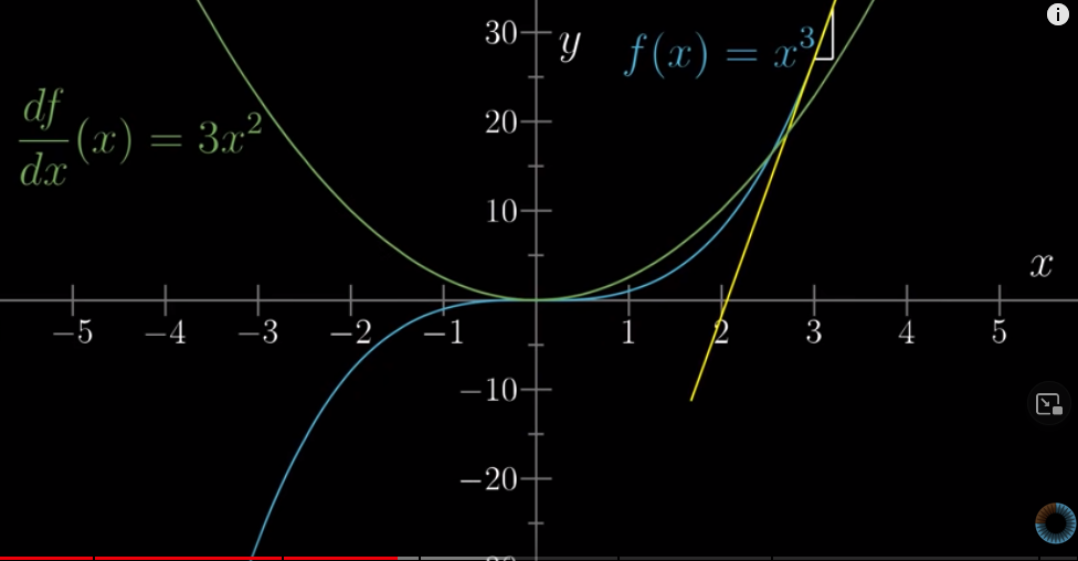
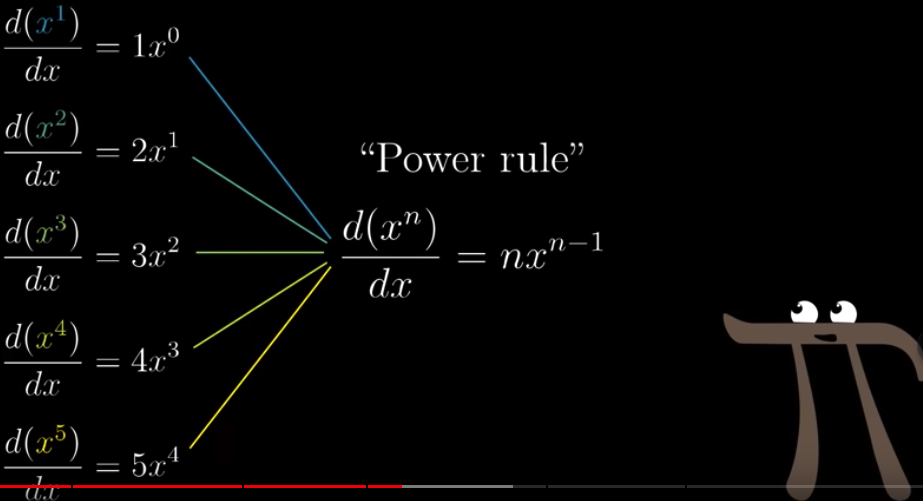
What this means is that in the graph of $f(x)=x^3$, the slope at any $x$ is exactly $3x^2$:

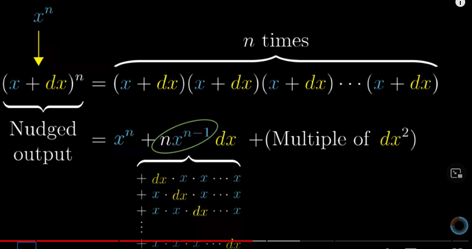
Based on this, we have the “power rule”:

For the derivative of $f(x) = \frac{1}{x}$: https://hongtaoh.com/en/2022/08/29/two-derivatives/

For the derivative of $f(x) = \sqrt{x}$: https://hongtaoh.com/en/2022/08/29/two-derivatives/

But I don’t understand the derivative of $sin(\theta)$. I’ll revisit it, maybe also look at https://www.khanacademy.org/math/ap-calculus-ab/ab-differentiation-1-new/ab-diff-1-optional/v/derivative-of-sin-x?modal=1

Lesson 4: Visualizing the chain rule and product rule #

The previous lessons are on how to compute the derivative for a single function, but how about combined functions?

There are three ways to combine two or more functions:

1. Add them together, e.g., $sin(x) + x^2$
2. Multplication, e.g., $sin(x)x^2$
3. Throw one into another, called “function composition”, e.g., $sin(x^2)$

Let’s compute their derivatives.

Sum rule #

First, $f(x) = sin(x) + x^2$. Let’s say $g(x) = sin(x)$ and $h(x) = x^2$. So, $f(x) = g(x) + h(x)$. If we have an increase in $x$: $dx$. Then the associated increase in $sin(x)$ is $dg = sin(x+dx) - sin(x) = cos(x)dx$. Why? Because

$$\frac{dg}{dx} = cos(x)$$

Similarly, we have:

$$\frac{dh}{dx} = 2x$$

Therefore, we have

$$df = dg + dh = cos(x)dx + 2x\cdot dx$$ So

$$\frac{df}{dx} = cos(x) + 2x$$

That is to say, when we add two functions, the derivative of this combined function is the sum of each individual derivative.

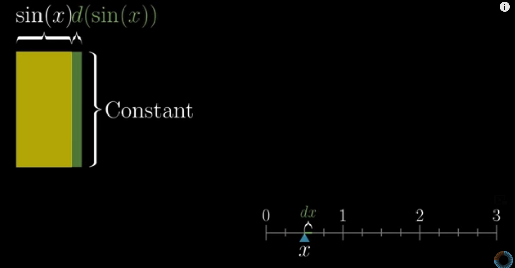
Product rule #

Let’s look at the product of the two functions: $$f(x) = g(x)h(x)$$

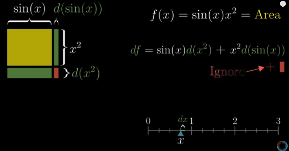
We can think of the product of $g(x)$ and $h(x)$ as the area of a rectangle. When we have a tiny increase of $dx$, then we have an associated increase of $dg$ and $dh$ in $g(x)$ and $h(x)$ respectively. We have proved that $dg = cos(x)dx$ and $dh = 2xdx$. So the increase in the “area” is:

$$\begin{aligned} df &= dg\cdot x^2 + dh\cdot sin(x) + dg\cdot dh \\ &= cos(x)dx\cdot x^2 + 2xdx\cdot sin(x) + cos(x)dx\cdot 2xdx \\ \end{aligned}$$ Then we devide it by $dx$ to calculate the derivative:

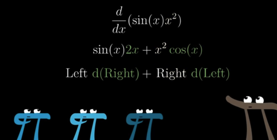
$$\frac{df}{dx} = cos(x)x^2 + 2x\cdot sin(x) + cos(x)\cdot 2xdx$$ Because $dx$ is approaching zero, we can safely ignore $cos(x)\cdot 2xdx$ and conclud that the derivative of $f(x)=g(x)h(x)$ is

$$\frac{df}{dx} = cos(x)x^2 + 2x\cdot sin(x)$$

This can be memorized as

Then what about the derivative of $f(x) = 2g(x)$?

We have:

$$df = 2dg$$

Because $dg = cos(x)dx$, we have:

$$\frac{df}{dx} = \frac{2dg}{dx} = 2cos(x)$$

Yeah, that’s the derivative. When we multiply a function by a constant, the derivative of this new function is the product of this constant and the derivative of the original function.

Chain rule #

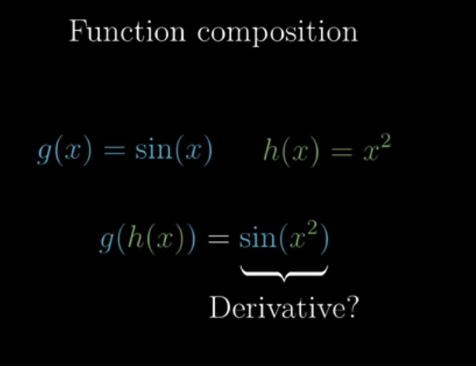
For $f(x) = g(h(x))$, we can represent it as:

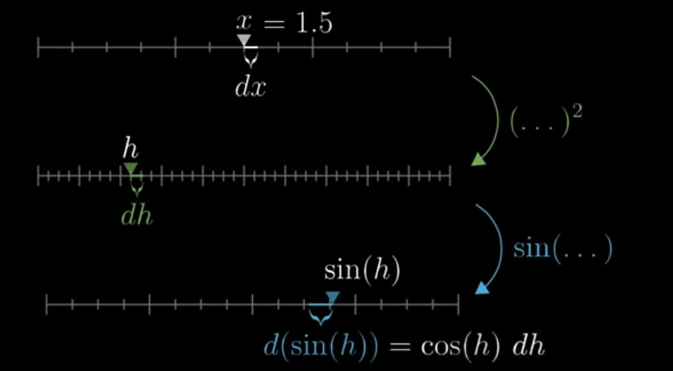
In $f(x) = g(h(x))$, when we have an increase of $dx$, the increase in $h(x)$ is $dh = 2xdx$ because $h(x) = x^2$. That’s easy to understand. Then, let’s look at the whole function, $g(h(x))$. Let’s represent $h(x)$ as $h$. Because $g(h) = sin(h)$, we have $dg = cos(h)dh = cos(h)2xdx$.

Because $f(x) = g(h)$, we have:

$$\frac{df}{dx} = \frac{dg}{dx}=cos(h)2x=cos(x^2)2x$$

So we know that if $f(x) = g(h(x))$, then the derivate of $f(x)$ is $dOuter(inner)\cdot dInner$.

Lesson 5: What’s so special about Euler’s number e #

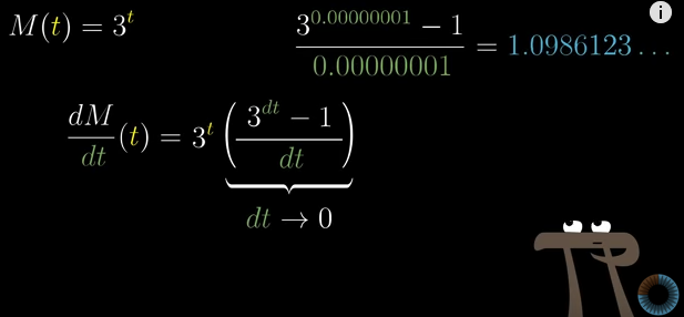
What’s the derivative of $f(t) = 2^t$?

Let’s see:

$$df = 2^{t+dt} - 2^t = 2^t2^{dt} - 2^t = (2^{dt} - 1) 2^t$$

So we have:

$$\frac{df}{dt} = 2^t \cdot \frac{2^{dt}-1}{dt}$$

As $dt$ approaches zero, we will find that $\frac{2^{dt}-1}{dt}$ is approaching a constant:

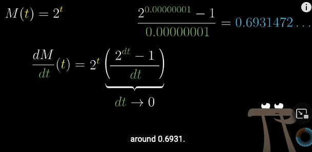
Therefore, the derivative of $2^t$ is itself multiplied by a constant.

The same is for $3^t$ and $8^t$, just that the constant is different:

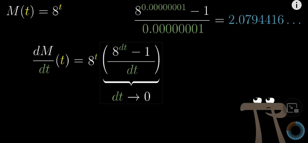
And you may notice this as well:

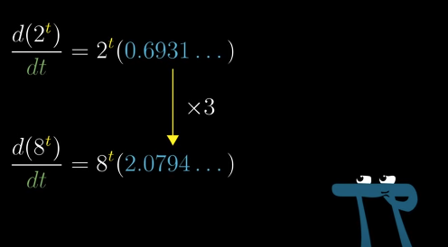
One interesting question is whether there is a base, denoted as $e$ and the derivative of $e^t$ is itself multiplied by $1$. There is. And that’s the definition of $e$.

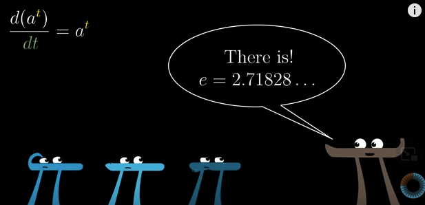
With this, we can gain a deeper understanding of what we have observed above.

If you remember the chain rule, you’ll know that the derivative of $e^{ct}$ where $c$ is a constant, is $c\cdot e^{ct}$.

Then, we define $ln(m)$ as “e to the degree of what equals m”. Then,

$$2^t = e^{ln(2)t}$$

This is because $2 = e^{ln(2)}$, and $(e^2)^t = e^{2t}$.

And we know the derivative should be $ln(2) e^{ln(2)t} = ln(2)\cdot2^t$.

And indeed, $ln(2)$ is that constant around $0.6931$.

What this tells us is that the derivative of $c^t$ is $ln(c)\cdot c^t$.

By the way,

$$ln(2) = log_e^{(2)}$$

Chapter 6: Implicit differentiation #

To be finished:

https://www.youtube.com/watch?v=qb40J4N1fa4&list=PLZHQObOWTQDMsr9K-rj53DwVRMYO3t5Yr&index=6

Chapter 7 Definition of and Computing limits #

Formal definition of a derivative #

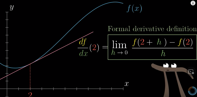
Compute limits with L’Hopital’s rule #

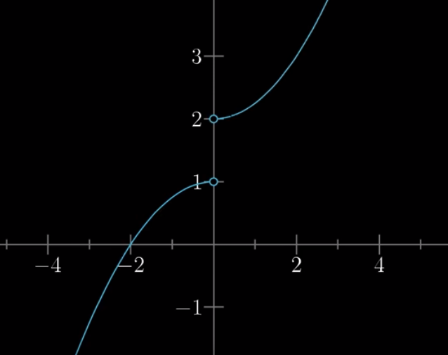
First, plot this function:

$$f(x) = \frac{(2+x)^3 - 2^3}{x}$$

y <- function(x) {
  ((2+x)^3 - 2^3)/x
}

curve(y, from = -8, to = 2, xlab = 'x', ylab='y')

The result will be:

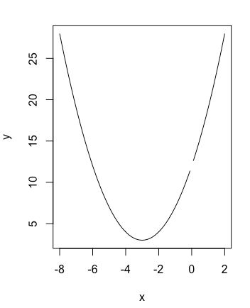
You see that the function is not defined at $x=0$. What if I ask you, when $x$ approaches 0, which value is $y$ approaching?

You may say we can compute the derivative of $f(x)$. But, what for? The derivative tells you the slope of the tangent line at $x=0$. However, since $f(0)$ is not even defined, there is no tangent line at $x=0$ at all.

Dead end.

We can, instead, think of this question this way. $f(0)$ is not defined, okay, fine. But what if we have a tiny change in $x$: $dx$. We can compute $f(dx)$, and this is where $f(0)$ is approaching, right? Then, the question now is, what is the value of $f(dx)$?

If $g(x) = (2+x)^3 - 2^3$ and $h(x) = x$, we have:

$$f(x) = \frac{g(x)}{h(x)}$$

So

$$f(dx) = \frac{g(dx)}{h(dx)}$$

Now, let’s plot $g(x)$ and $h(x)$ first:

Using R:

y1 <- function(x) {(2+x)^3 - 2^3}
y2 <- function(x) {x}
curve(y1, from = -4, to = 1, xlab = 'x', ylab='y', col='red')
curve(y2, col='blue', add=TRUE)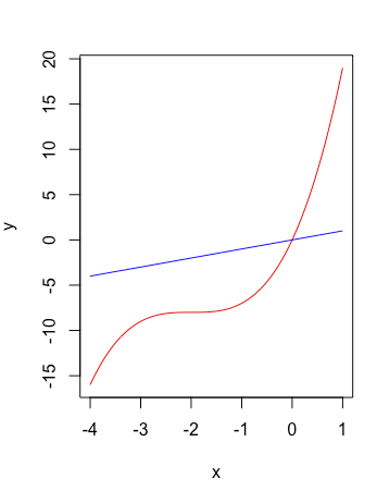

We see that $g(0) = h(0) = 0$.

When $x=0$ and we have a tiny increase of $dx$, the associated change in $g(x)$ will be:

$$dg = g(0+dx) - g(0) = g(dx) - 0 = g(dx)$$

Because $g(x) = (2+3)^3 - 8$, we know that:

$$\frac{dg}{dx} = 3 \cdot (x+2)^2$$

So $g(dx) = dg = 3 \cdot (x+2)^2 \cdot dx$

When $x=0$ and we have a tiny increase of $dx$, the associated change in $h(x)$ will be:

$$dh = h(0+dx) - h(0) = h(dx) - 0 = h(dx)$$

Because $h(x) = x$, we know that

$$\frac{dh}{dx} = 1$$ We have $h(dx) = dh = dx$

So

$$f(dx) = \frac{g(dx)}{h(dx)} = \frac{dg}{dh} = \frac{3 \cdot (x+2)^2 \cdot dx}{dx} = 3 \cdot (x+2)^2$$

Plug in $x=0$ and we have $f(dx) = 3 \times 2^2 = 12$. So $f(x)$ is approaching 12 at $x=0$.

$(\epsilon, \delta)$ definition of of limits #

Some limits are defined whereas others are not. For example,

$$\lim_{x \to 0} f(x) = \frac{(2+x)^3 - 2^3}{x}$$

is defined whereas

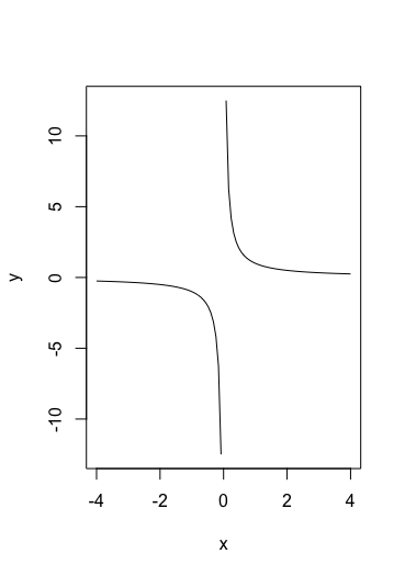
$$\lim_{x \to 0} g(x) = \frac{1}{x}$$ is not.

Why? And how can you tell whether a limit is defined or not?

The plot for $f(x)$:

The plot for $g(x)$:

I think Khan Academy explains the $(\epsilon, \delta)$ definition of of limits really well: you give me the number $\epsilon$ which indicates how close you want to be to the limit of $f(x)$ as $x$ approaches $c$, which is denoted as $L$, and I can find a number $\delta$ such that if $x$ is within $\delta$ of $c$, then $f(x)$ is within $\epsilon$ of $L$.

This can be done for $f(x)$ but not for $g(x)$ because in $g(x)$, $L$ is indefinite.

Similarly, limit in the following function at $x=0$ is not defined as well:

This is because, for example, if $\epsilon = 0.5$, and let’s say $f(1.8) = 2.5$. Can you find a $\delta$ such that

if $|x - 0| < \delta$, then $|f(x) - L| < 0.5$? (See here )

You might say $L = 2$ and $\delta = 1.8-0 = 1.8$. However, when $-1.8 < x < 0$, is $|f(x) - L| < 0.5$? No.

Chapter 8 Integration and the fundamental theorem of calculus #

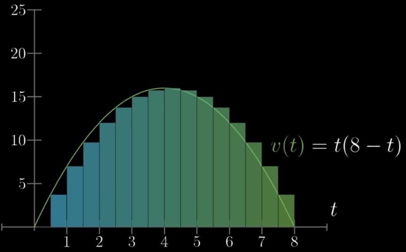
This is the plot of the speed of a car moving as a function of time:

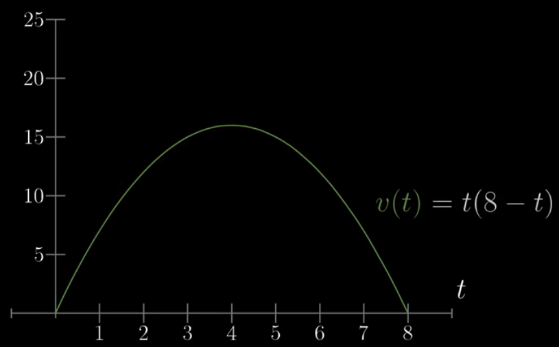
Based on this, I ask you, could you tell me the distance the car has covered at certain time, say, $t = 4s$?

That’s hard to solve, but let’s say the car’s speed is 0 from 0s to 1s, 7 from 1s to 2s, 12 from 2s to 3s, …:

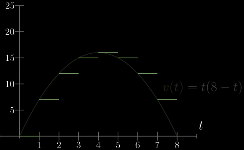
Then, the distance the car has covered at $t=3$ is the area of the first three bars (the first bar being empty):

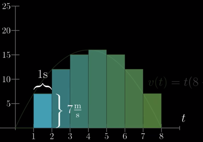
When we have smaller and smaller time gaps:

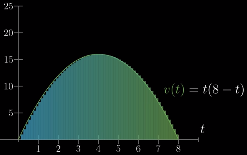
We will know that at any time of $t$, the distance the car has travelled is the area between $v(0)$ and $v(t)$.

We can view the area as a function of time: $s(T)$. We also call this the integral of $v(t)$. When we have a tiny change in time, denoted as $dT$, the associated change in area, or distance, denoted as $ds$, can be approximated as $v(T) \cdot dT$.

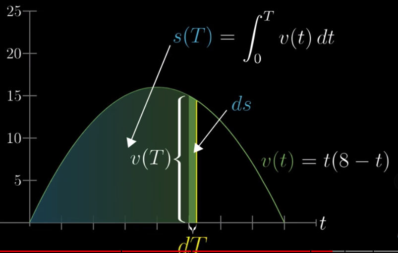
So

$$\frac{ds}{dT} = v(T)$$

Therefore, the derivative of $s(T)$ is $v(T)$. This, in fact, applies to every function: the derivative of the integral of a function is the function itself.

We know the derivative of $s(T)$ is $v(T)$ and we know $v(t)$. Then, the question is, what function has a derivative of $v(t) = t(8-t)$?

We know that it can be this

$$s(t) = 4t^2 - \frac{1}{3}t^3 + c$$ where $c$ is a constant.

In our case, we know that $t = 0$ because $s(0) = 0$. But, in other case, we might not know this but this shouldn’t be a problem because if we want to know the distance travelled between $t=5$ and $t=0$, we just $s(5) - s(0)$ and this cancels out the effect of the unknown $c$.

In the above example:

Where we know $v(t)$, and we want to know the area between $v(0)$ and $v(T)$, how to represent this mathematically?

$$\int_0^T = v(t)dt$$ and $dt$ is approaching 0.

Chapter 9 What does area have to do with slope #

Given this:

I ask you, what is the average of distance travelled from $t=0$ to $t=4$?

Imagine have very small $dt$:

Then the average distance will the sum of heights of all the small bars, divided by the number of bars up until $t=4$.

How many bars do we have until $t=4$:

$$N = \frac{4}{dt}$$

So:

$$\bar{s} = \frac{\sum bars}{N} = \frac{\sum bars \times dt}{4} = \frac{\int_0^4 v(t)dt}{4} = \frac{s(4) - s(0)}{4}$$ We know $s(t) = 4t^2 - \frac{1}{3}t^3$.

It’s plot is:

y <- function(x) {
  4*x^2 - 1/3*x^3
}

curve(y, from = 0, to = 8, xlab = 't', ylab='s')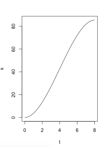

You can see that $\frac{s(4) - s(0)}{4}$ is the slope:

y <- function(x) {
  4*x^2 - 1/3*x^3
}

curve(y, from = 0, to = 8, xlab = 't', ylab='s')

y1 <- function(x) {
  y = 256 * x / 24  
}

curve(y1, from = 0, to = 4, add=TRUE, col="red")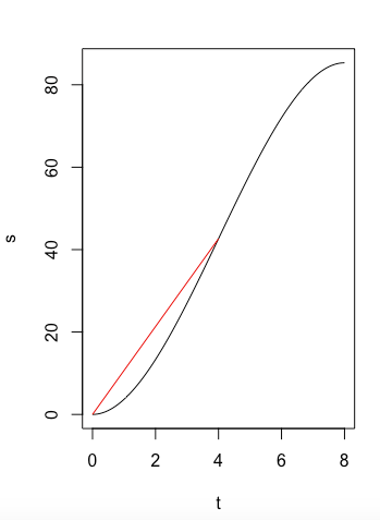

When you think about it, you’ll realize that when we ask about the average distance travelled between $t=0$ and $t=4$, we calculate the area, and divide it by the number of $dt$ we have. Because $v(t)$ is the derivative of $s(t)$, the average distance is equivalent to the average slope of many points between $t=0$ and $t=4$ for $s(t)$. And this average slope is the slope between two points: $t=0$ and $t=4$.

Chapter 11 Taylor series #

Taylor series is about approximating non-polynomial functions with polynomial functions near some inputs, say, $x=0$.

Let’s try approximating $f(x) = cos(x)$ with something like $h(x) = c_0 + c_1 x + c_2 x^2 + c_3 x^3 ...$

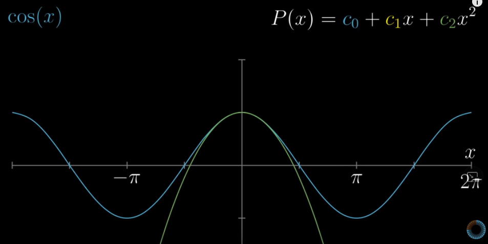
Because $cos(0) = 1$, $c_0 = 1$.

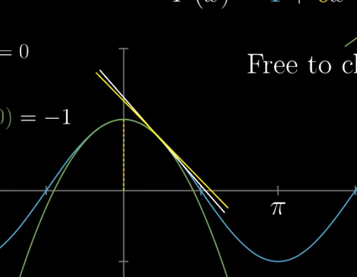
Then, to further approximate $f(x)$, it’s best if the tangent line at $f(0)$ is the same as that at $h(0)$. This means $f^{\prime}(0) = h^{\prime}(0)$. We know that $f^{\prime}(x) = sin(x)$, so $f^{\prime}(0) = sin(0) = 0$. Because $h^{\prime}(x) = c_1 + 2c_2 x + 3c_3 x^2 + ...$, we know that $c_1 = 0$.

The tangent line at $f(0)$ indicates the rate of change for $f(x)$ at $0$. Even though the rate of change itself is $0$, the rate of change for that rate of change, i.e., the second derivative, is decreasing at $x=0$. The second derivative is $-cos(x)$, which is $-cos(0) = -1$ at $x=0$.

To approximate $f(x)$, it’s best if the second derivative of $h(x)$ is the same. The second derivative of $h(x)$ is $2c_2 + 2\cdot3 c_3 x + ...$. So we have $c_2 = - \frac{1}{2}$.

Making sure that $f(x)$ and $h(x)$ share the same second derivative means that these two functions “curve at the same rate”, i.e., the slope of the polynomial does not move more quickly (or slowly) than that of $f(x)$ at points nearing $x=0$:

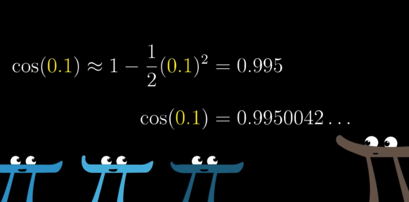
We can stop here, and approximate $f(x) = cos(x)$ with

$$h(x) = 1 - \frac{1}{2}x^2$$

Let’s see:

When you watch the process closely, you’ll see that at the level of first derivative, all elements before $c_1$ will disappear and all elements after $c_1$ will be $0$ if we plug in $x=0$. That’s why we can easily calculate $c_1$.

For example, this is when we calculate $c_1$:

$$c_1 + 2c_2 x + 3c_3 x^2 + ...$$

This is when we calculate $c_2$:

$$2\cdot 1 c_2 + 3 \cdot 2 c_3x + ...$$

This is when we calcualte $c_3$:

$$3\cdot2\cdot1c_3 + 4\cdot3\cdot2\cdot1c_4x + ...$$

If we are approximating at inputs other than 0, say, at $x=\pi$, we can do this:

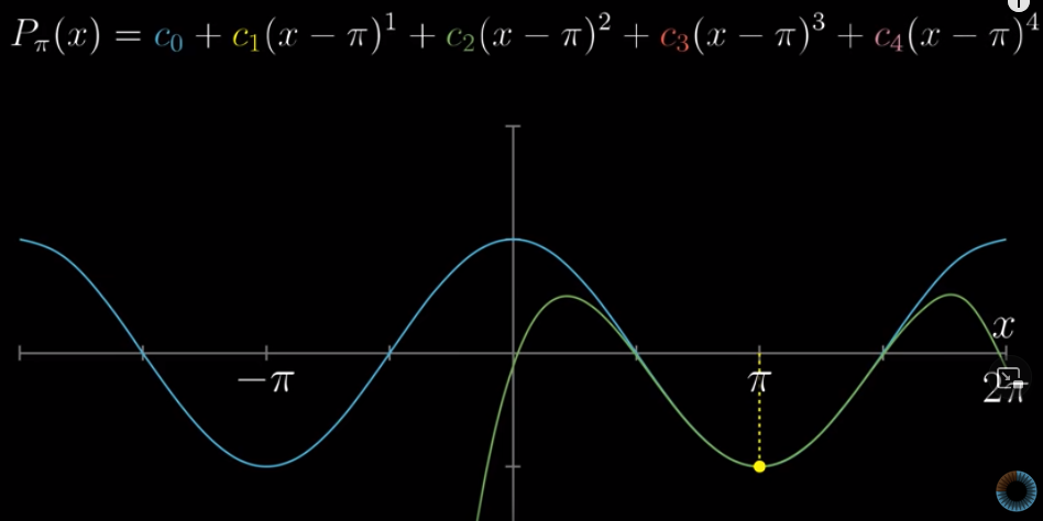
By the way, this is how we represent second derivative at $x=0$:

$$\frac{d^2f}{dx^2}(0)$$ You can do similar things for third, fourth, fifth derivatives.

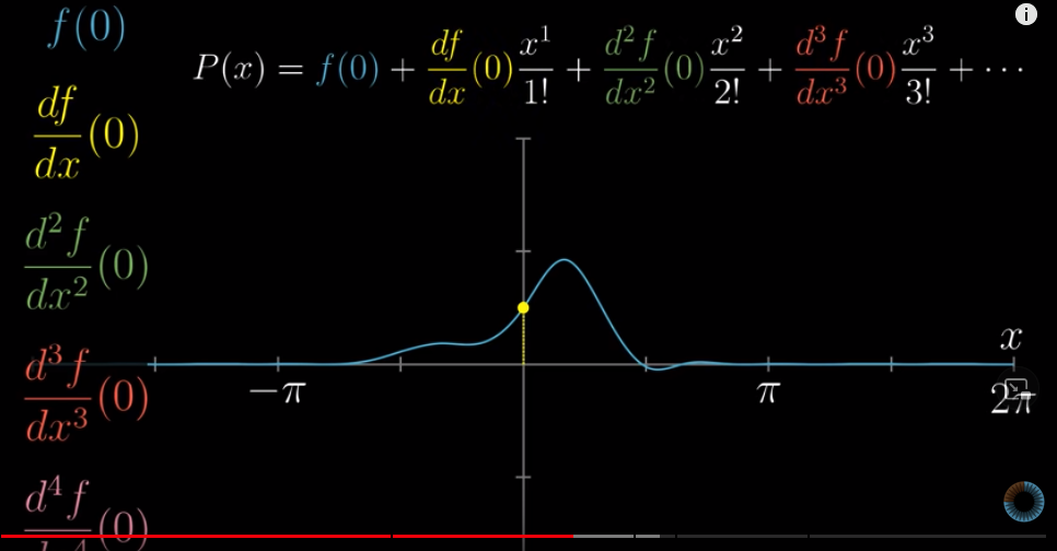
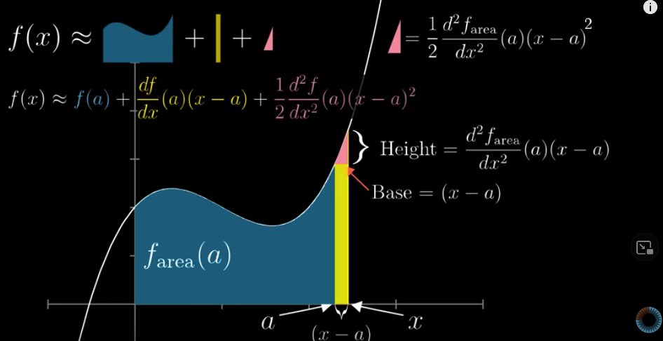
This is the more general representation of Taylor Series:

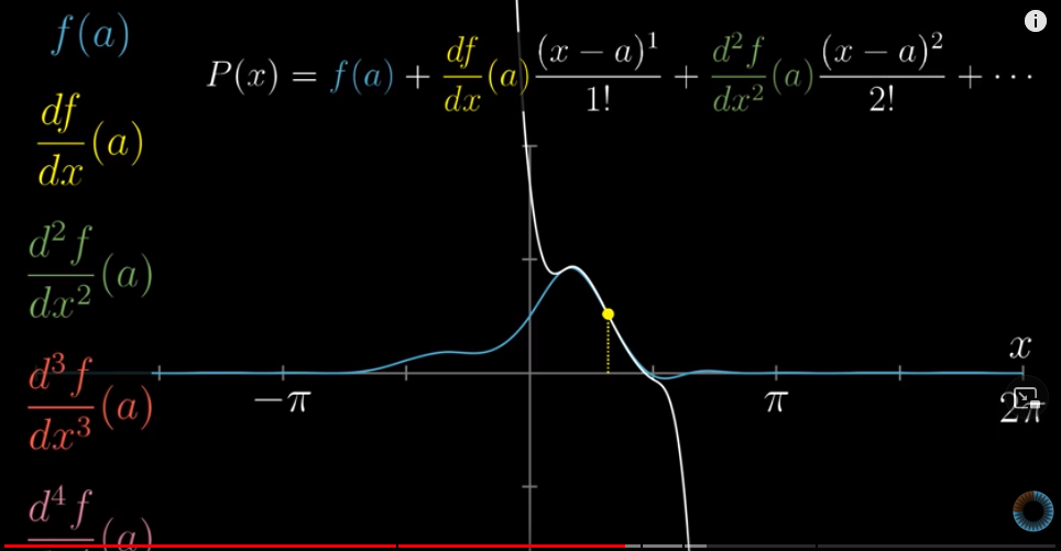
Or, more generally

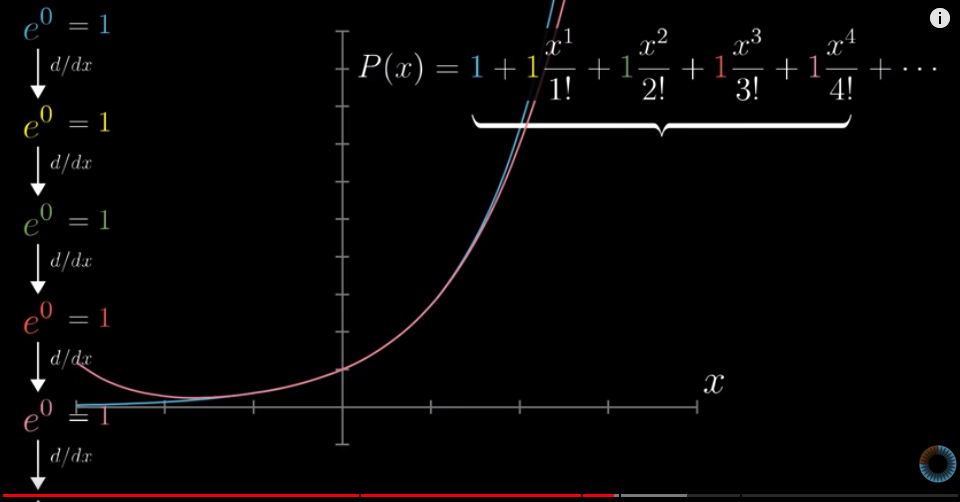
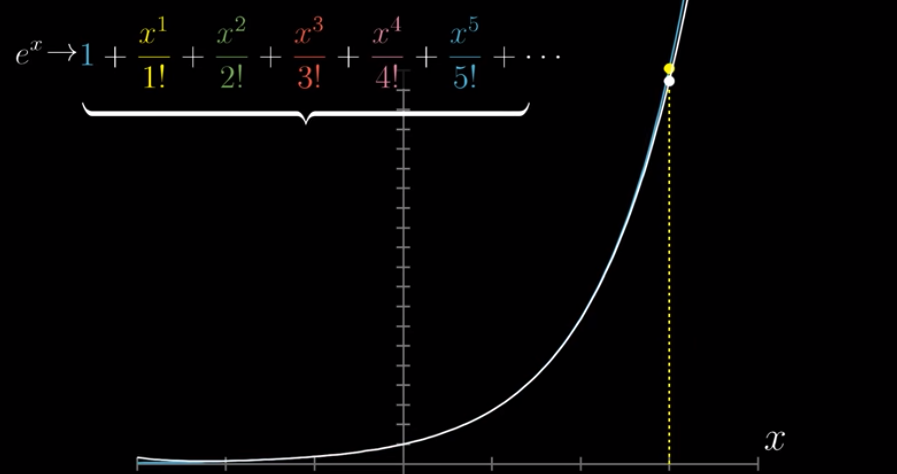
This is the Taylor polynomials for $e^x$:

This is the graphical meaning of the second derivative:

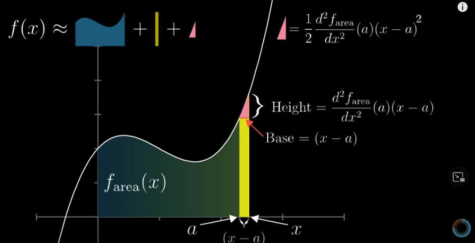
The Base is easy to understand. What about the height? Well, you know that $f(x)$ is the derative of $f_{area}(x)$. The slope of $f(x)$ is $\frac{f(x) - f(a)}{x-a} = \frac{Height}{x-a}$. Therefore, the Height is $slope \times (x-a)$. The slope is the derivative of $f(x)$, so it is also the second derivative of $f_{area}(x)$.

The area of the pink triangle is the same as that in the general representation of Taylor polynomials:

$$\frac{d^2f}{dx^2}(a)\frac{x^2}{2!}$$

If we know $f(a)$, how can we approximate $f(x)$ with polynomials:

Converging versus diverging #

For $e^x$, Taylor series is approaching $e^x$ at any given $x$:

But that’s not always the case. For example, for this function, Taylor series is only approaching the function for inputs within a certain interval, for example, the natural log $ln(x)$:

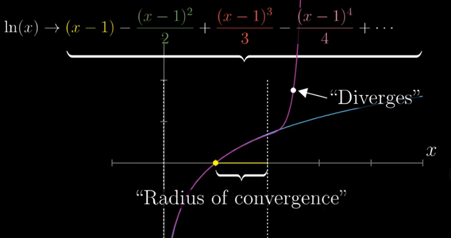
The approximation diverges for inputs $x>2$.

The distance vetween the input you are using, and the maximum input where the series do converge (instead of diverging), is called the Radius of convergence.

Last modified on 2022-09-30