Lesson 0: Preview #
We focused too much on numeric understanding and did not focus on geometrical understanding. Geometric understanding of linear algebra is important because it quickly gives us a sense of how to use it in different settings.
Lesson 1: Vectors #
Physics students think that vectors are arrows pointing in space. Two elements: length and direction. You can move the vectors around and they can still be the same vectors. Vectors can be 2-dimentional or 3-dimentional.
Computer science students think vectors are ordered lists of numbers. For example:
$$\begin{bmatrix} 2,600 \ {ft}^2 \\ 3,000 \ USD \end{bmatrix}$$Math students think that as long as it can be added to another vector or that it can be multiplied by a number, then it is a vector.
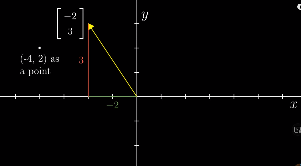
When thinking of a vector, think of an arrow in a 2-d coordinate system with its start sitting on the origin.
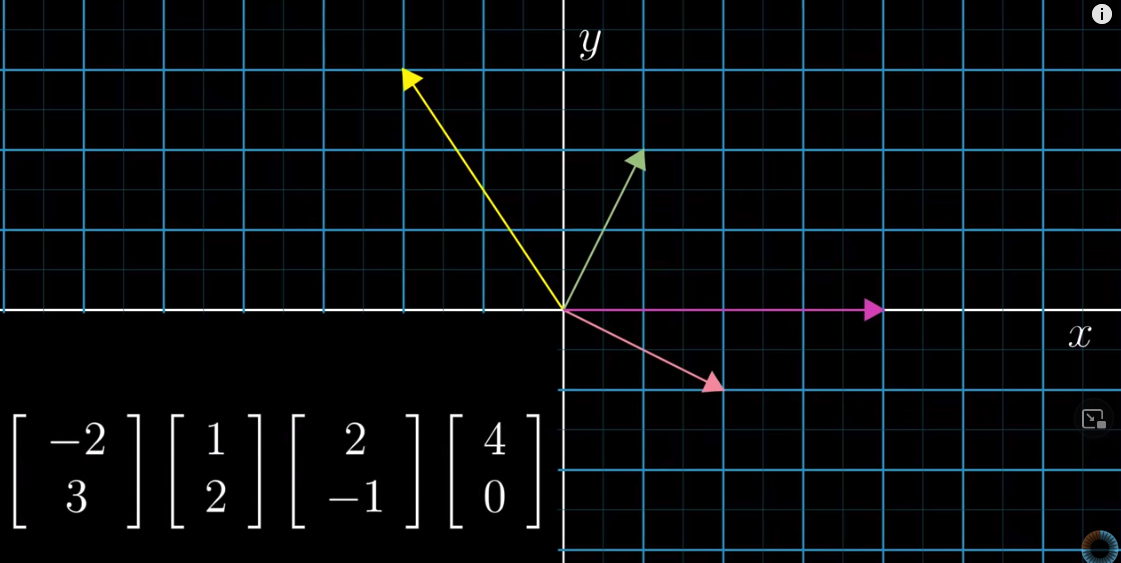
Note that writing the coordinates horizontally denotes a point. To denote a vector, we write the two coordinates vertically.
Vectors in 3 dimenion is basically the same as those in two dimension; only that in 3 d, there is a Z axis.
Addition and multiplication #
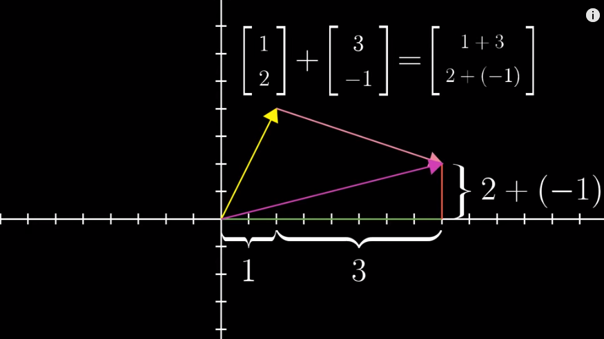
Adding one vector (A) to another one (B) means moving A towards B such that the tail of B sits at the tip of A:
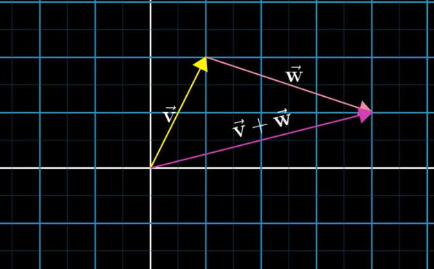
But why? Why the addition of vectors is defined this way but not another? We can think of vectors as something that represents certain movements (which contain (1) a direction and (2) steps). The result of the addition of B to A is the result of A movement + B movement.
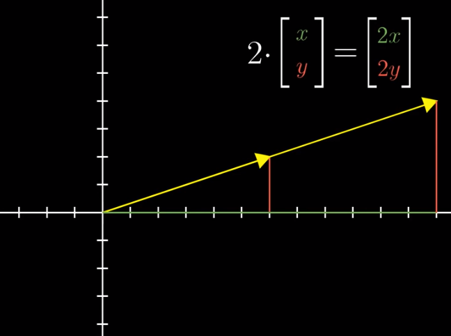
Multiplication of a vector by a number is easy to understand. Stretching or squishing is called “scaling”. And that number is called a “scalar”.
Lesson 2: Linear combinations, span, and basis vectors #
You have a simple vector, say
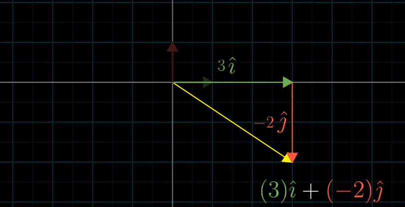
$$\begin{bmatrix} 3 \\ -2 \end{bmatrix}$$
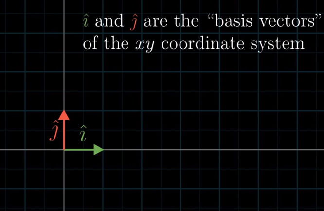
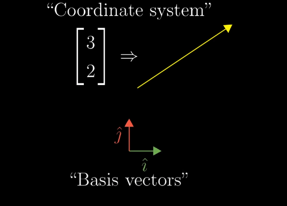
Think of it as the sum of $3\hat{i}$ and $-2\hat{j}$ where $\hat{i}$ is one unit right and $\hat{j}$ is one unit up. That is to say, think of the two numbers in the above vector as two scalars. $\hat{i}$ and $\hat{j}$ are called the “basis vectors” of the $xy$ coordinate system.
An interesting and important point to think about is what if we choose different “basis vectors”?
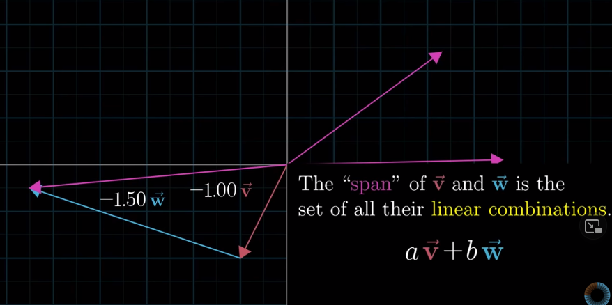
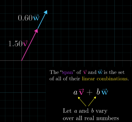
Linear combination of $\vec{v}$ and $\vec{w}$: scaling two vectors ($\vec{v}$ an $\vec{w}$) and adding them. (Hongtao: when you think about this definition again, you can see that linear combination includes two elements: scalar multiplication and vector addition)
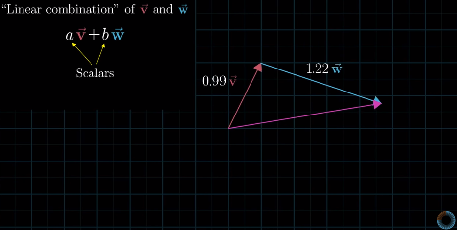
Span: the set of all possible vectors that the linear combination of $\vec{v}$ and $\vec{w}$ can reach.
If $\vec{v}$ and $\vec{w}$ line up, then the span is all the vectors along that line:
As we have talked about, linear algebra revolves around vector addition and scalar multiplication. “Span” is all the possible vectors that result from vector addition and scalar multiplication for a given pair of vectors, $\vec{v}$ and $\vec{w}$.
Arrows or points: if you are dealing with a specific vector, think of it as an arrow; if you are dealing with a set of or sets of vectors, think of each vector as a point (with its tail sitting at the origin of the $xy$ coordinate).
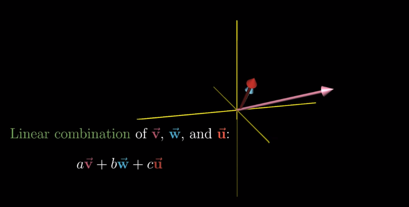
Linear combination in 3-d space is similarly defined:
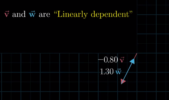
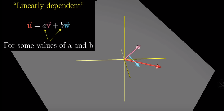
In 3-d if the third vector is sitting on the span of the first two, or in 2-d where the two vectors line up, then one vector is redundant in a way that it is not contributing to the “span”. Whenever we have a redundant vector, we call the vectors as “linearly dependent”.
In 3-d, if vectors are linearly dependent, one vector can be expressed as a linear combination of the other two vectors.
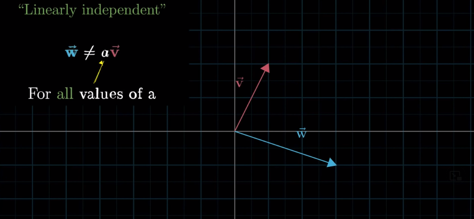
If there is no redundant vector, in other words, if every vector is adding to our “span”, then we say that these vectors are “linearly independent.”
Technical definition of “basis vectors”:
The basis of a vector space is a set of linearly indepdent vectors that span the full space.
Lesson 3: Linear transformation and matrices #
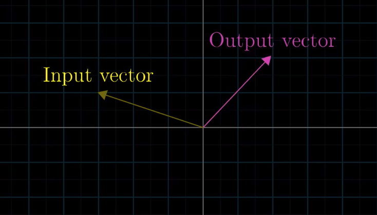
Transformation simply means “function”: it takes in inputs and spits out outputs. In the context of linear algebra, the function takes in a vector and spits out another vector.
Transformation differs from “function” in that it denotes some “movements”: the input vector “moving into” the output vector:
Arbitrary transformations are complicated.
![]()
Fortunately, in linear algebra, we only focus on “linear transformations”.
A transformation is linear if it has two properties:
- Lines remain straight lines (without getting curved)
- The origin remains in place.
This is not a linear transformation because lines are curved:

This is not a linear transformation either, because the origin moves:
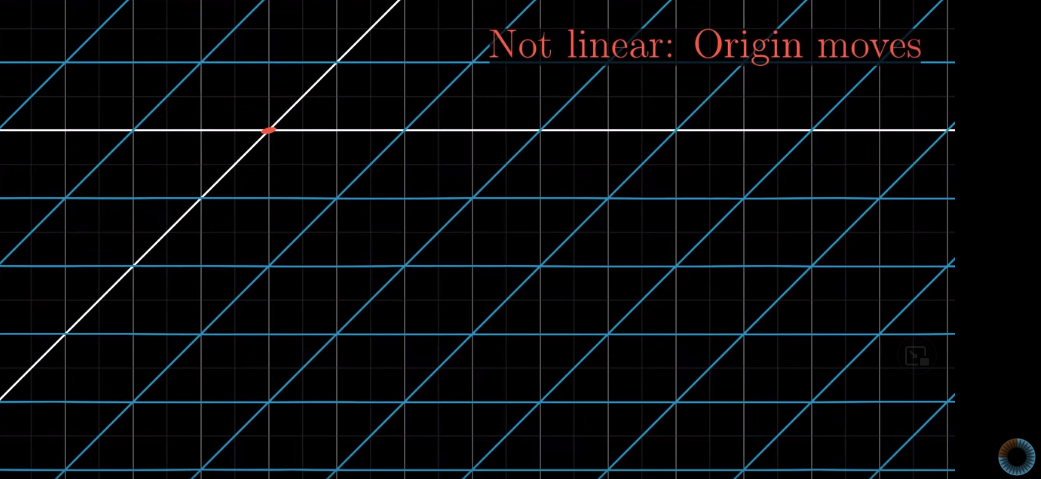
Sometimes, all lines seem to be lines, and the origin remains in place. However, the diagonal lines are curvy, so it is not a linear transformation:
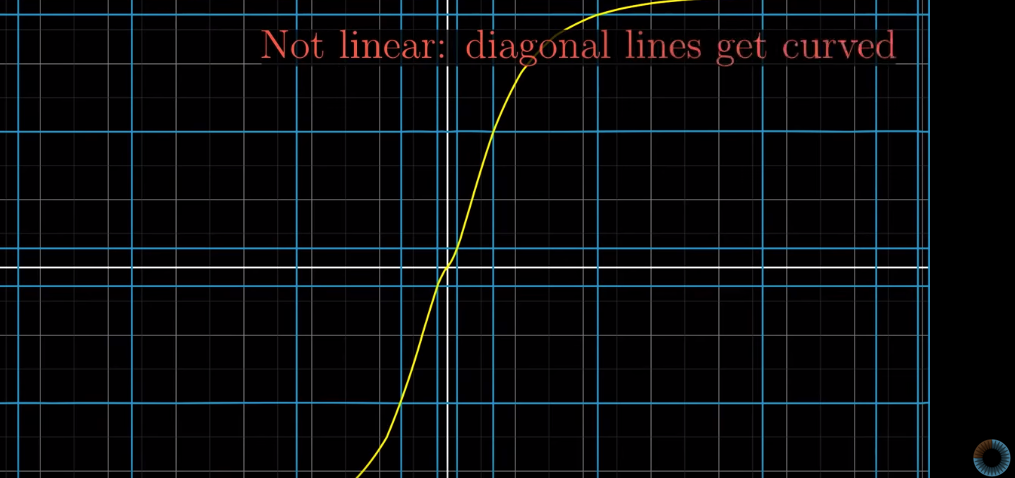
In linear transformations, grid lines “remain parallel and evenly spaced.”
Before going deeper into linear transformation, think about this question. Linear transformation is a like a function such that it takes in an input vector and spits out an output vector. The question is this: I give you an input vector of $\begin{bmatrix} x_{in} \\ y_{in}\end{bmatrix}$, what function can spit out the output vector of $\begin{bmatrix} x_{out} \\ y_{out}\end{bmatrix}$ ? Bascially, what I am asking is this: if the input vector has coordinates of (x,y), how to get its output coordinates (after linear transformation)?
![]()
The solution:
A very important property of linear transformation is that for any given vector, its linear combination remains the same afer linear transformation. For example, if we have $\vec{v} = -1\hat{i} + 2 \hat{j}$, then after transformation, we will have this: $Transformed \vec{v} = -1(Transformed \hat{i}) + 2(Transformed \hat{j})$
![]()
After transformation:
![]()
It looks very simple, but this property of linear transformation is pretty important. Why and how?
If we know that the linear combination remains the same, then in order to know where $Transformed \vec{v}$ lands, we only need to know the coordinates of $Transformed \hat{i}$ and $Transformed \hat{j}$.
If the coordinates of $Transformed \hat{i}$ in the original grid are (1, 2) and $Transformed \hat{j}$ is at (3,0), then we know that $Transformed \vec{v}$ must be at (5,2):
$-1*(1,2) + 2*(3,0) = (5,2)$
![]()
We have the above calculations because the original $\vec{v}$ is $\begin{bmatrix} -1 \\ 2 \end{bmatrix}$, but $\vec{v}$ can be anything: $\begin{bmatrix} x \\ y \end{bmatrix}$. If we know that $Transformed \hat{i}$ is $\begin{bmatrix} 1 \\ -2 \end{bmatrix}$ and $Transformed \hat{i}$ is $\begin{bmatrix} 3 \\ 0 \end{bmatrix}$, then for each vector, we can know where it lands after transformation using this formula:
![]()
We can combine the coordinates of $Transformed \hat{i}$ and those $Transformed \hat{j}$ into a $2\times2$ matrix:
$$\begin{bmatrix} 1 & 3\\ -2 & 0 \end{bmatrix}$$
Then, if you have a $\vec{v} = \begin{bmatrix} x \\ y \end{bmatrix}$, and you have $Transformed \hat{i}$ and $Transformed \hat{j}$ shown above, you can know the coordinates of $Transformed \vec{v}$ this way:
$$x\begin{bmatrix} 1 \\ -2 \end{bmatrix} + y\begin{bmatrix} 3 \\ 0 \end{bmatrix}$$
To be more general, suppose the $2\times2$ matrix is $\begin{bmatrix} a & b\\ c & d \end{bmatrix}$ where (a,c) are coordinates of $Transformed \hat{i}$ and (b, d) are coordinates of $Transformed \hat{j}$. For any given vector $\begin{bmatrix} x \\y \end{bmatrix}$, we can compute its coordinates after two-dimensional linear transformation this way:
![]()
One important take-away from this lection is that we can consider every matrix as a certain transformation of space. For examlple, $\begin{bmatrix} 1 & 3 \\ 2 & 1 \end{bmatrix}$ is the result of moving $\hat{i}$ (1,0) to (1,2) and moving $\hat{j}$ (0,1) to (3,1):
![]()
This point is extremely important if you want to get a deeper understanding of linear algebra.
Shear #
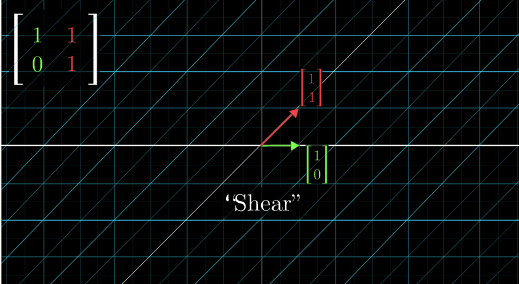
By the way, if we keep the x-axis in place and tilt the y-axis 45 degrees to the right, this transformation is called “shear”.
Lesson 4: Matrix multiplication as composition #
Matrix multiplication #
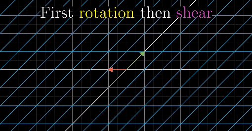
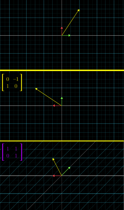
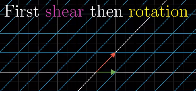
What if we have two linear transformations in a sequence? For example, first rotate 90 degrees counterclockwise and then do a shear.
The original position:
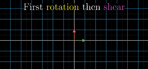
Step 1: Rotate 90 degrees counterclockwise:
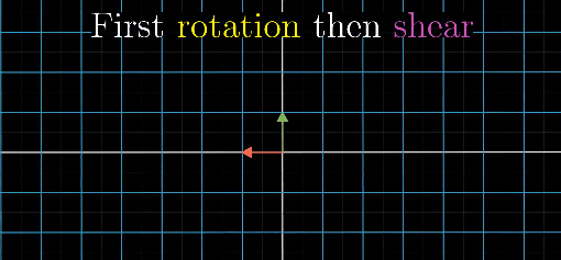
Step 2: Shear:
Then, I’ll ask you, how to represent the above transformations matematically?
Step 1 is easy. We can represent the linear transformation using this matrix:
$$\begin{bmatrix} 0 & -1 \\ 1 & 0\end{bmatrix}$$
But, how about Step 2?
You may say this:
$$\begin{bmatrix} 1 & -1 \\ 1 & 0\end{bmatrix}$$
Because that is the final stage. However, this is not a correct representation of Step 2. This is because that final stage is the result of two steps: 90 degree rotation and then shear, rather than Step 2 (i.e., shear) alone. But how to represent Step 2 itself?
We got stuck. We don’t know how to represent “shear”. In Lesson 3, shear is defined this way: keep the x-axis in place and tilt the y-axis 45 degrees to the right. And it is represented as this:
$$\begin{bmatrix} 1 & 1 \\ 0 & 1\end{bmatrix}$$
Here, you may start wondering: wait, is Step 2 really a “shear”? Shouldn’t a “shear” be keeping x-axis in place and tilting the y-axis? In Step 2, it seems that what is tilted is the x-axis (which is in green), not the y-axis (in red). Why do we call it a “shear”?
Good question! Now, you know why we find it difficult to represent Step 2 mathmatically.
Here, I want to reiterate a very important point: The essense of linear transformation is about transforming the space, and matrix is a way to let us know how that space is being transformed.
If you look at Step 2 closely, you’ll find that the transformation is the same as that when we define “Shear” in Lesson 3, right? The “movement” feels the same, right?
What is different in Step 2, from the definition of “shear”, lies in the starting point. In Step 2, the starting point seems to be $\begin{bmatrix} 0 & -1 \\ 1 & 0\end{bmatrix}$, which is the result of Step 1. However, when we define “Shear”, the starting point is $\begin{bmatrix} 1 & 0 \\ 0 & 1 \end{bmatrix}$.
Here is the problem: if we do not have the same starting point, then it’s impossible to mathematically represent a linear transformation.
For example, in the definition of shear, the mathematical representation of the transformation, or of the “movement” is $\begin{bmatrix} 1 & 1 \\ 0 & 1\end{bmatrix}$. But this representation makes sense, i.e., tells us what that movement is, only if we know that the starting point is $\begin{bmatrix} 1 & 0 \\ 0 & 1 \end{bmatrix}$. The starting point of Step 2 is $\begin{bmatrix} 0 & -1 \\ 1 & 0\end{bmatrix}$. Then, it’s impossible to mathematically represent the linear transformation using a single matrix, as other people don’t know what the starting point is.
This is very easy to solve: We can stipulate that, for a representation of a linear transformation, its starting point must be $\begin{bmatrix} 1 & 0 \\ 0 & 1 \end{bmatrix}$. That is to say, to represent a linear transformation mathematically, we only need to show where $\begin{bmatrix} 1 & 0 \\ 0 & 1 \end{bmatrix}$ lands after the transformation. Therefore, the representation of Step 2 is the same as the definition of “Shear”: $\begin{bmatrix} 1 & 1 \\ 0 & 1\end{bmatrix}$.
This, in fact, makes sense. Think about it: for Step 2, the “movement” from $\begin{bmatrix} 0 & -1 \\ 1 & 0\end{bmatrix}$ to $\begin{bmatrix} 1 & -1 \\ 1 & 0\end{bmatrix}$ is the same as that from $\begin{bmatrix} 1 & 0 \\ 0 & 1 \end{bmatrix}$ to $\begin{bmatrix} 1 & 1 \\ 0 & 1\end{bmatrix}$. Right?
Thus, the two steps are these:
This is the final result:
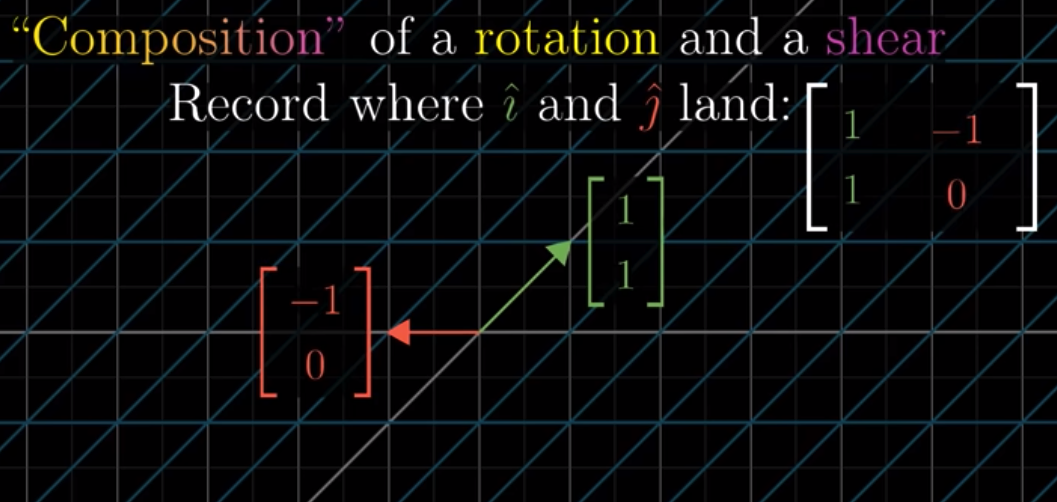
We call the final result, $\begin{bmatrix} 1 & -1 \\ 1 & 0\end{bmatrix}$, as the composition of Step 1 and Step 2. This is the defintion of the multiplication, or product, of two linear transformations, or, two matrices. We can consider this composition as a linear transformation itself, which can be represented as a matrix: $\begin{bmatrix} 1 & -1 \\ 1 & 0\end{bmatrix}$.
We can represent the multiplication as this:
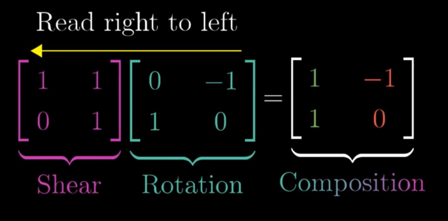
On the left panel, we write and read from right to left. That is to say, if we first apply a rotation and then a shear, then it should be written in the above fashion.
The above should be calculated this way.
The first coumn will be:
$$\begin{bmatrix} 1 & 1 \\ 0 & 1\end{bmatrix} \begin{bmatrix} 0 \\ 1\end{bmatrix} = 0\begin{bmatrix} 1 \\ 0 \end{bmatrix} + 1 \begin{bmatrix} 1 \\ 1 \end{bmatrix} = \begin{bmatrix} 1 \\ 1 \end{bmatrix}$$
And the second column will be
$$\begin{bmatrix} 1 & 1 \\ 0 & 1\end{bmatrix} \begin{bmatrix}-1\\ 0 \end{bmatrix} = -1\begin{bmatrix} 1\\ 0 \end{bmatrix} + 0 \begin{bmatrix} 1\\ 1 \end{bmatrix} = \begin{bmatrix} -1\\ 0 \end{bmatrix}$$
Therefore we have:
$$\begin{bmatrix} 1 & 1 \\ 0 & 1\end{bmatrix} \begin{bmatrix} 0 & -1 \\ 1 & 0 \end{bmatrix} = \begin{bmatrix} 1 & -1 \\ 1 & 0\end{bmatrix}$$
What the above is calculating is where Transformed $\hat{i}$ and Transformed $\hat{j}$ land after two linear transformations (first rotation and then shear). To do that, we can think about it this way. After Rotation, Transformed $\hat{i}$ is $\begin{bmatrix} 0 \\ 1 \end{bmatrix}$, and Transformed $\hat{j}$ is $\begin{bmatrix}-1\\ 0 \end{bmatrix}$. After applying a shear, Transformed $\hat{i}$ moves to $\begin{bmatrix} 1 & 1 \\ 0 & 1\end{bmatrix} \begin{bmatrix} 0 \\ 1\end{bmatrix} = \begin{bmatrix} 1\\ 1 \end{bmatrix}$, and Transformed $\hat{j}$ moves to $\begin{bmatrix} 1 & 1 \\ 0 & 1\end{bmatrix} \begin{bmatrix}-1\\ 0 \end{bmatrix} = \begin{bmatrix}-1\\ 0 \end{bmatrix}$.
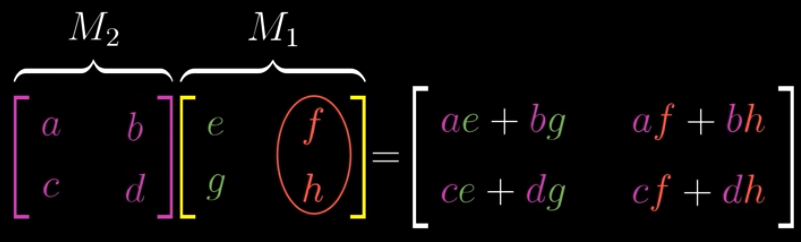
This is the calculations in general:
$$\begin{bmatrix} a & b \\ c & d\end{bmatrix} \begin{bmatrix} e & f \\ g & h\end{bmatrix}$$
The first column of the result will be:
$$\begin{bmatrix} a & b \\ c & d\end{bmatrix} \begin{bmatrix} e \\ g\end{bmatrix} = \begin{bmatrix} a \\ c \end{bmatrix}e + \begin{bmatrix} b \\ d\end{bmatrix}g$$
The second column of the result will be:
$$\begin{bmatrix} a & b \\ c & d\end{bmatrix} \begin{bmatrix} f \\ h\end{bmatrix} = \begin{bmatrix} a \\ c \end{bmatrix}f + \begin{bmatrix} b \\ d\end{bmatrix}h$$
Noncommutativity #
One question is: does the order of matrices matter in matrix multiplication?

Let’s take a look.
If we first take a shear, and then do the 90 degree rotation:
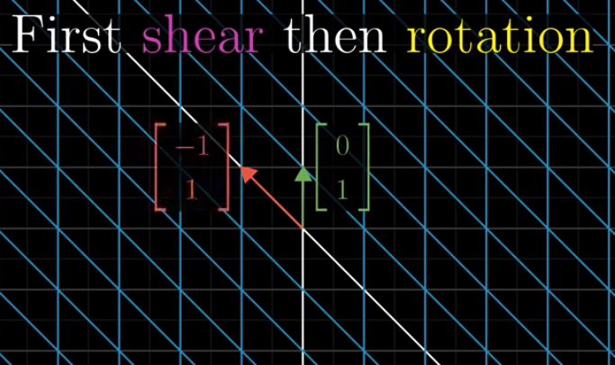
We can see that the results are different.
Therefore, order matters:

Of course they aren’t equal:
$$\begin{bmatrix} 1 & 1 \\ 0 & 1\end{bmatrix} \begin{bmatrix} 0 & -1 \\ 1 & 0\end{bmatrix} \neq \begin{bmatrix} 0 & -1 \\ 1 & 0\end{bmatrix} \begin{bmatrix} 1 & 1 \\ 0 & 1\end{bmatrix}$$
Associativity #
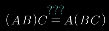
Yes. The two are equal.
Lesson 5: three-dimensional linear transformations #
![]()
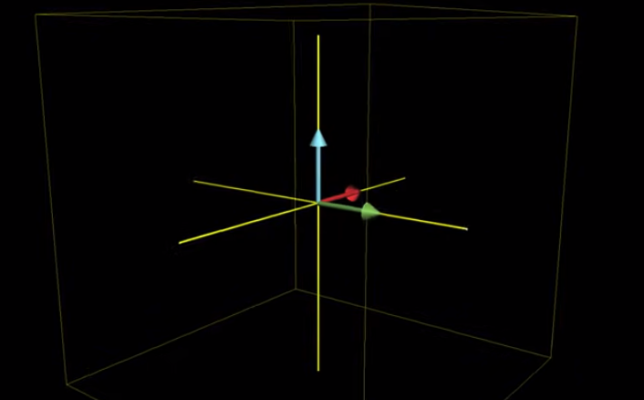
We added one basis vector in a 3d space: $\hat{k}$ which is in the Z direction.
For linear transformations in a 3d space, grid lines also need to be parellel and evenly spaced, and the origin needs to remain in place as well.
Multiply a vector by a matrix #
For a vector $\vec{v}$ in 3d space, how to calculate its positions after a linear transformation?
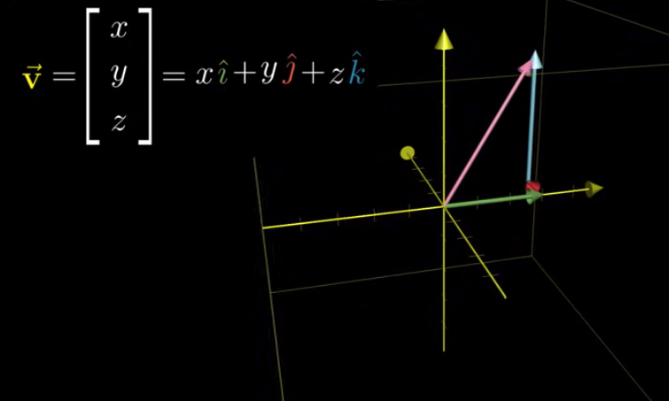
It’s almost the same. Each element in $\vec{v}$ represents how we should multiple, or scale, a corresponding basis vector.
After transformation, the scalars remain the same:
![]()
Note that in the Transformation matrix, the left column is Transformed $\hat{i}$, the middle column is Transformed $\hat{j}$, and the last column is Transformed $\hat{k}$.
Matrix multiplication #
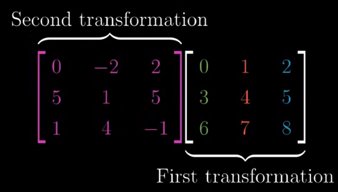
It’s the same as matrix multiplication in a 2d space.
The result should be
$$\begin{bmatrix} 6 & 6 & 6 \\ 33 & 44 & 55 \\ 6 & 10 & 14\end{bmatrix}$$
If you use R, you compute it this way:
data1 <- c(0,5,1,-2,1,4,2,5,-1)
a <- matrix(data1, nrow = 3, ncol = 3)
data2 <- c(0,3,6,1,4,7,2,5,8)
b <- matrix(data2, nrow = 3, ncol = 3)
a %*% b
Lesson 6: determinant #
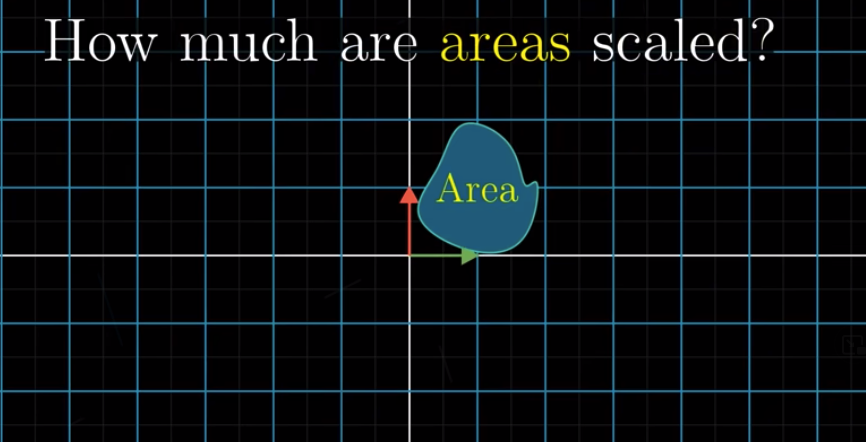
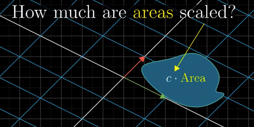
Some linear transformations stretch out space whereas others squash it. Then how can we describe this? How can we describe the degree to which the space is being changed?
We can measure this by looking at how much a given area is being changed after linear transformation.
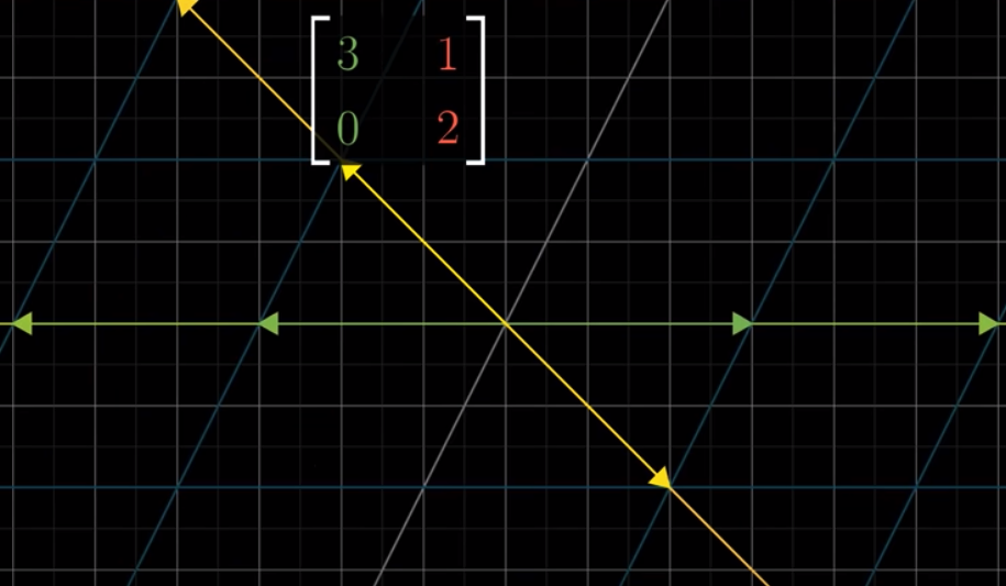
Let’s take a concrete example: $\begin{bmatrix} 3 & 0 \\ 0 & 2\end{bmatrix}$.

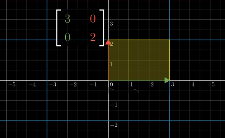
We can see that the area was 1 before the transformation and changes to 6 after the transformation. Therefore, the area is scaled up by a factor of 6. The determinant of this transformation is 6.
What about a shear?
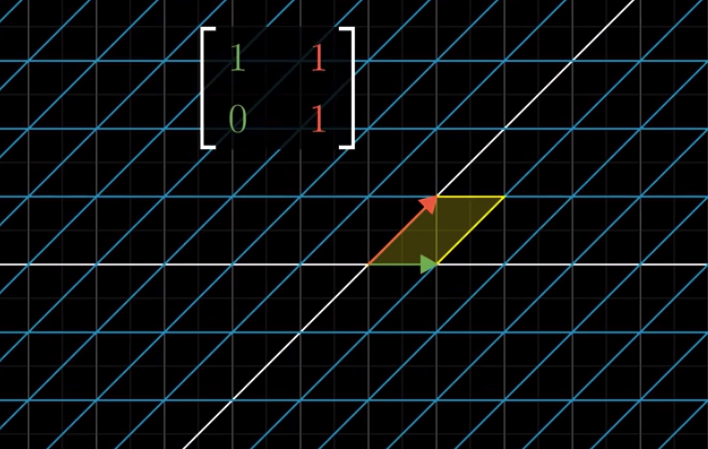
It became a parallelogram with an area of 1. Therefore, the determinant of a shear transformation is 1.
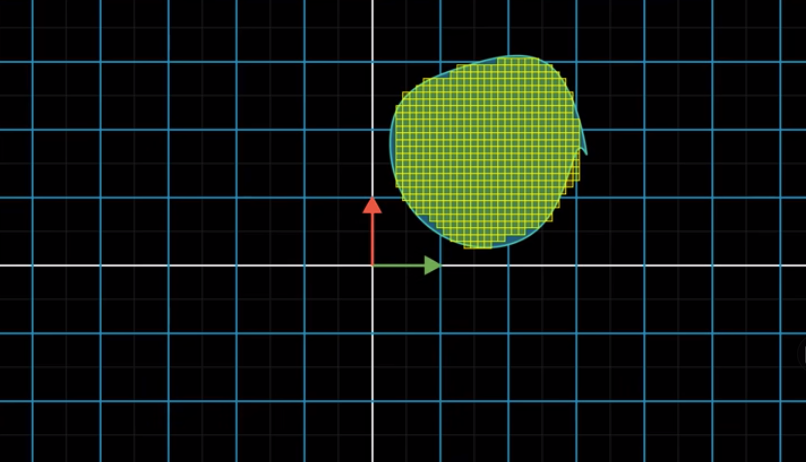
If we know how the unit square changes, we will know how any area in the space changes.
If the area is a square, then its change, in terms of the scaling factor, is the same as the unit square.
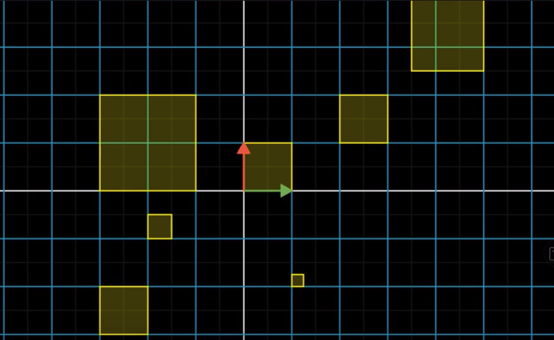
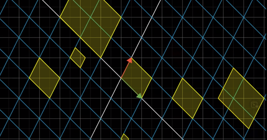
Then, areas that are not squares can be approximated by squares:
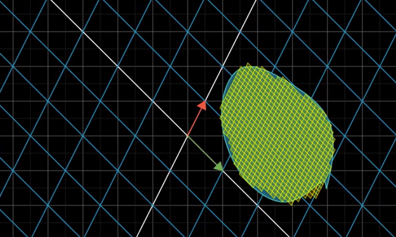
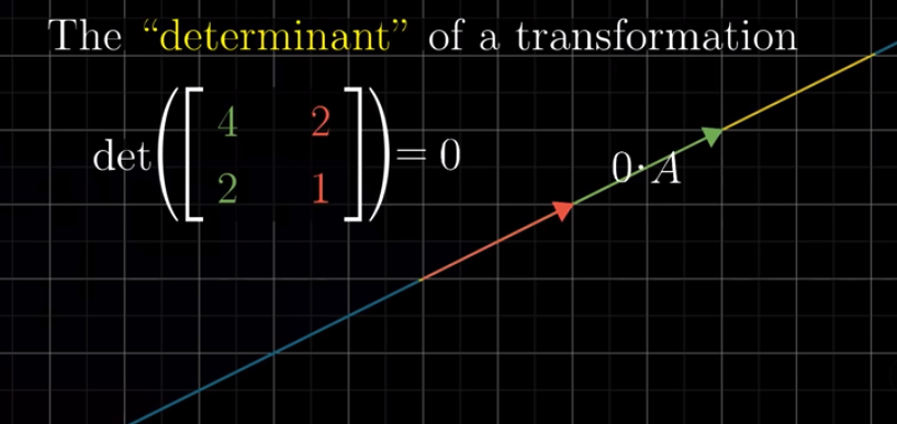
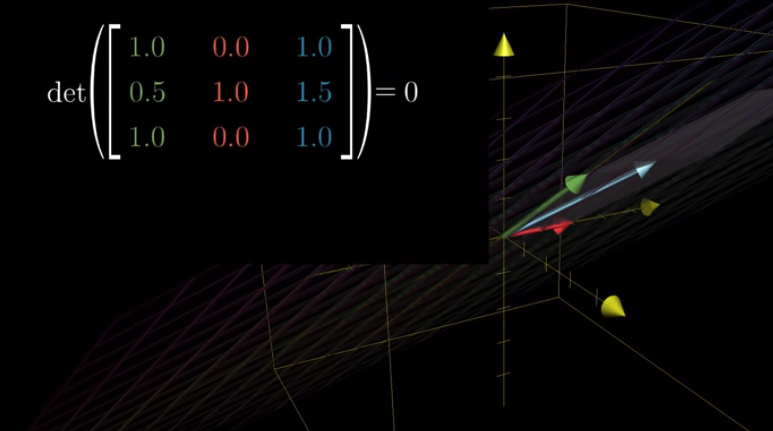
Note that the determinant of a transformation is 0 if Transformed $\hat{i}$ and Transformed $\hat{j}$ are linearly dependent. For example:
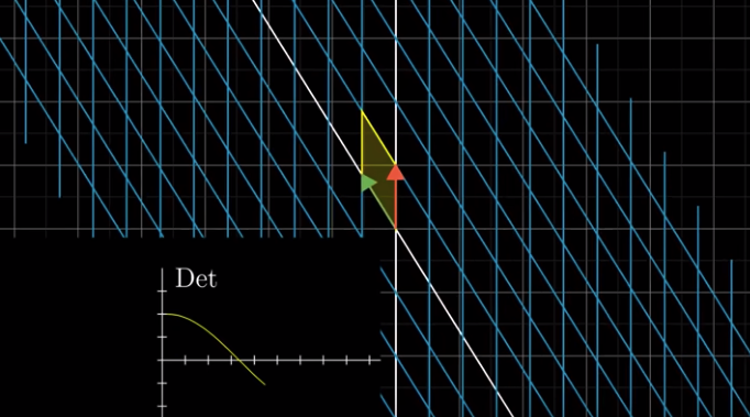
The sign of a determinant #
The definition of determinant actually allows negative determinants. But what does the sign, i.e., + or -, mean?
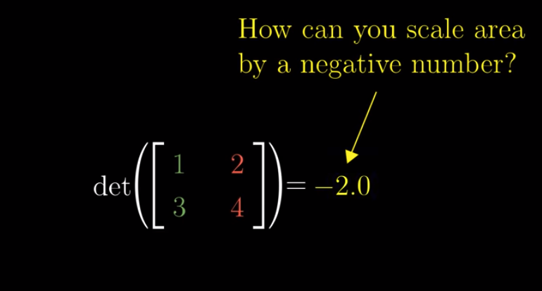
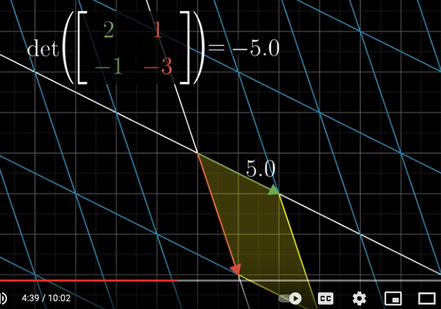
The sign of a determinant is all about orientation. After transformation, if Transformed $\hat{j}$ is still on the left of Transformed $\hat{i}$, then the sign is positive. Otherwise, it is negative. If Transformed $\hat{i}$ and Transformed $\hat{j}$ line up, then the determinant, of course, is 0.
When the determinant is negative, the transformation is like flipping the space over:
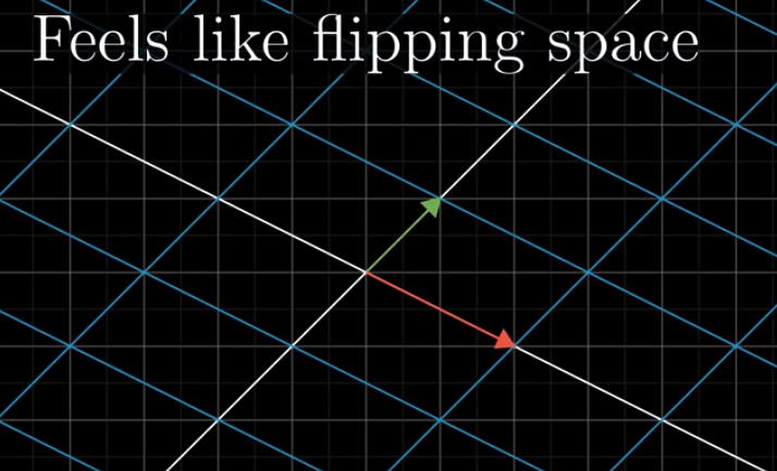
We call this as “inverting the orientation of space.”
The absolute value of the determinant indicates how much the space scales up or shrinks.
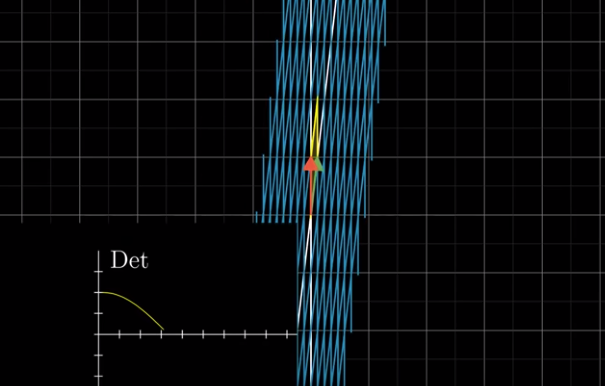
But why the sign indicates the orientation?
We can think of it this way. Imagine that we let $\hat{i}$ slowly approach $\hat{j}$. We can imagine that before they line up, the determinant keeps decreasing. When they do line up, the determinant becomes zero. Then, as $\hat{i}$ keeps moving away from $\hat{j}$ (and the sapce is being flipped), isn’t it natural that we let the determinant keep going down and become below zero, i.e., negative?
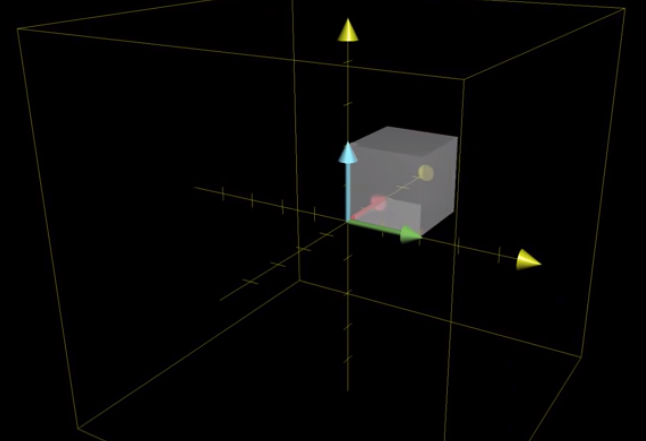
Determinant of a 3-D linear transformation #
The determinant of a 2-D linear transformation is about scaling areas; It is about scaling volumes in 3-D linear transformations.
To know the determinant, we look at how the unit cube whose edges are the basis vectors, changes in volume.
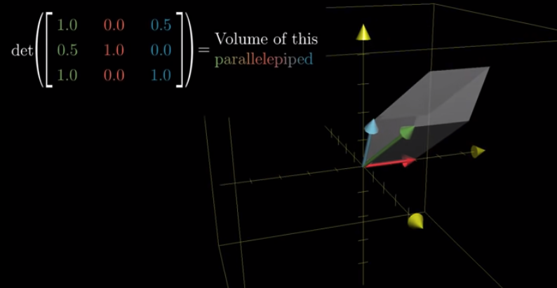
We call the object after transformation as parallelepiped.
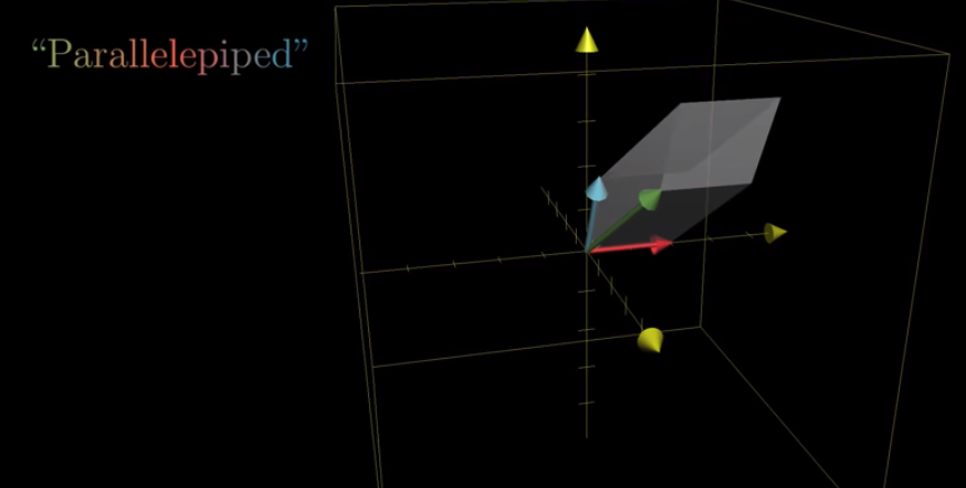
Because the volume of the cube is intially 1. To calculate the determinant, we only need to know the volume of the parallelepiped that the cube becomes.
If the determinant is 0, it means the space becomes a plane, a line, or even a single point.
Then what does the sign of the determinant mean? It still means the orientation, but how do we interpret it?
We can use the right hand rule.
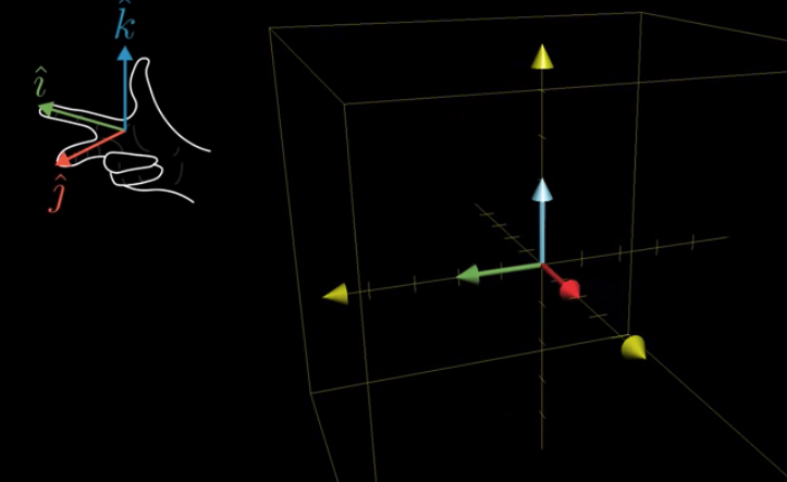
If you do the above with your right hand, then the sign should be positive. Otherwise, it is negative.
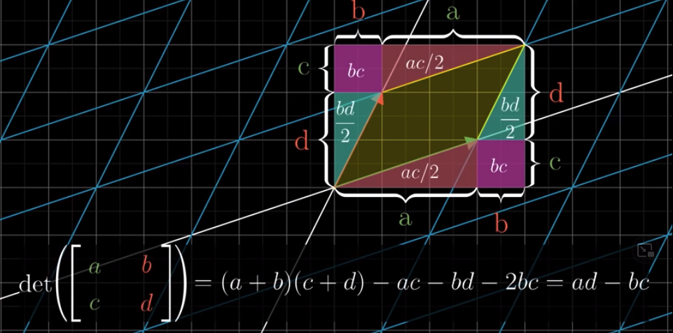
Determinant calculation #
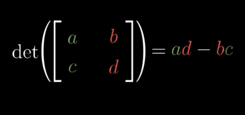
Why?
At the end of video, 3blue1brown asks us to prove this:
$$det(M_1M_2) = det(M_1)det(M_2)$$
Let’s first look at the left hand side. We first apply $M_2$ and then $M_1$. Suppose $M_2$ scale an area by $e$. After $M_2$, the unit area becomes $e$. Then we apply $M_1$. Be aware that the reference coordinates of $M_1$ are still the original coordinates (i.e., those before the application of $M_2$). Suppose $M_1$ will scale an area by $f$. Then a unit area will become $ef$ after applying $M_2$ and then $M_1$. That is to say, $det(M_1M_2) = ef$.
On the right hand side, $det(M_1) = f$ and $det(M_2) = e$. Therefore, $det(M_1)det(M_2) = fe = ef$. Therefore, we have $det(M_1M_2) = det(M_1)det(M_2)$.
One interesting thing is that:
$$det(M_2M_1) = ef = det(M_1M_2) = fe$$
Therefore, although the order matters for matrix multiplication, it does not matter if we are considering the determinant of the two.
The above discussion is based on the comments, below 3blue1brown’s original video (Lesson 6), by Kiran Kumar Kailasam and Ying Fan .
Lesson 7: Inverse matrices, column space, rank, and null space #
Inverse matrices #
Linear algebra is useful when describing the manipulation of the space. It can also help us solve “linear system of equations.”
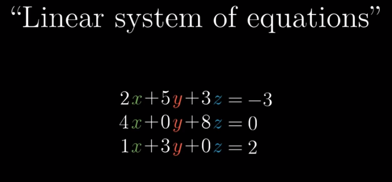
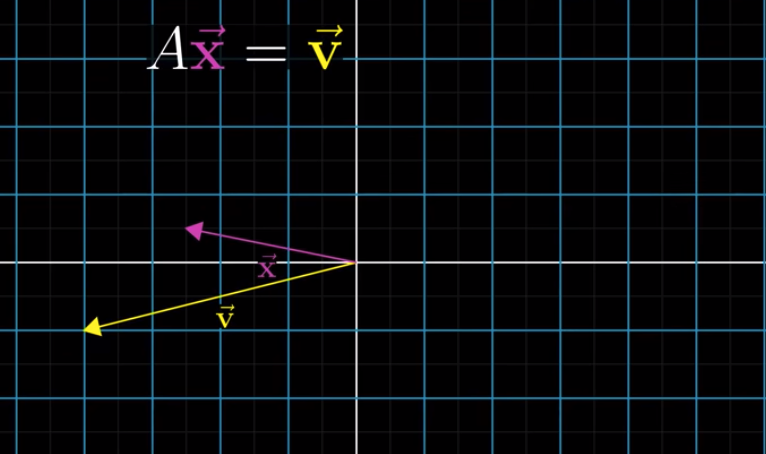
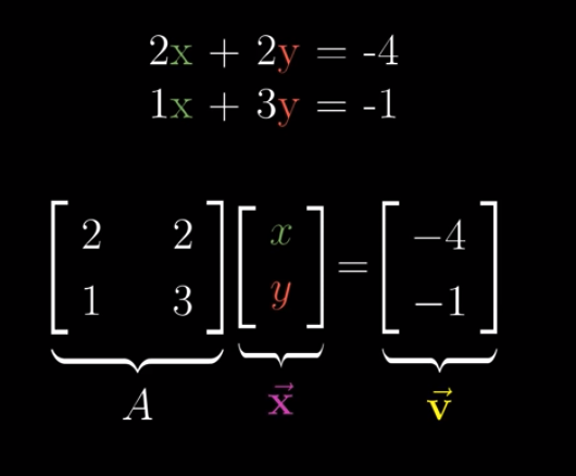
How? We can compare a linear system of equations with a linear transformation this way:
![]()
$\vec{x}$ here is the input vector, $A$ is the matrix denoting a transformation, and $\vec{v}$ is the output vector. Our goal, therefore, is to look for the $\vec{x}$, which, after applying a linear transformation described by $A$, lands on $\vec{v}$.
Let’s first assume that $det(A) \neq 0$. We will come back and talk about what if $det(A) = 0$ later.
Let’s take a simple case as an example.
To find out what $\vec{x}$ is, how about we applying another linear transformation, and let $\vec{v}$ lands on $\vec{x}$?
This linear transformation, which allows a transformed vector to go back to its original state, has a name: inverse transformation.
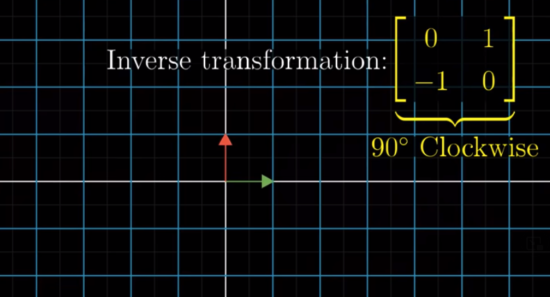
Let’s take a simple example. If $A$ is a counterclockwise 90 degree rotation:
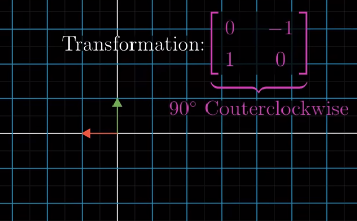
Then, the inverse of $A$, denoted as $A^{-1}$ is a clockwise 90 degree rotation:
Therefore, for any vector $\vec{m}$, if we first apply $A$ and then $A^{-1}$, then $\vec{m}$ reamins in place. “Applying $A$ and then $A^{-1}$” is two transformations, whose result can be seen as one single linear transformation: $AA^{-1} = \begin{bmatrix} 1 & 0 \\ 0 & 1\end{bmatrix}$. We call this as an “identity transformation”. When we apply an identity transformation to a vector, this vector remains in place.
If $det(A) \neq 0$, then we can find one and only one inverse transformation, i.e., $A^{-1}$. Once we find it, we can apply it to $\vec{v}$, which also means we apply it to $A\vec{x}$ because we have $A\vec{x} = \vec{v}$:
$$A^{-1}A\vec{x} = A^{-1}\vec{v}$$
Because $AA^{-1} = \begin{bmatrix} 1 & 0 \\ 0 & 1\end{bmatrix}$ is the identity transformation, we have $AA^{-1}\vec{x} = \vec{x}$; therefore, we have:
$$\vec{x} = A^{-1}\vec{v}$$
We know $A$ (and therefore $A^{-1}$) and $\vec{v}$, so we can calculate $\vec{x}$ easily.
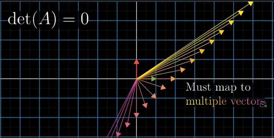
But what if $det(A) = 0$?
Let’s take one simple example. Let’s say $A = \begin{bmatrix} 1 & -1 \\ 0 & 0\end{bmatrix}$. Then we have $det(A) = 1\times0 - (-1)\times0 = 0$. Let’s say $\vec{x} = \begin{bmatrix} a \\ b\end{bmatrix}$. After applying $A$, $\vec{x}$ will land on $\vec{v} = \begin{bmatrix} a -b \\ 0\end{bmatrix}$.
Let’s say $a-b = 2$, which means $\vec{v} = \begin{bmatrix} 2 \\ 0\end{bmatrix}$. Then what’s $\vec{x}$? There are tens of thousands of possible versions of $\vec{x}$. For example, $\begin{bmatrix} 2 \\ 0\end{bmatrix}$, $\begin{bmatrix} 3 \\ 1\end{bmatrix}$, $\begin{bmatrix} 4 \\ 2\end{bmatrix}$, etc. If fact, as long as $a$ and $b$ are on the line of $y = x - 2$, they can be the coordinates of $\vec{x}$:
Therefore, if we are given $A$ and $\vec{v}$, and that $det(A) = 0$, we are not able to know what $\vec{x}$ is.
Let’s go back to how a linear system of equations is related to linear algebra:
In the example above, $A = \begin{bmatrix} 1 & -1 \\ 0 & 0\end{bmatrix}$ and $\vec{v} = \begin{bmatrix} 2 \\ 0 \end{bmatrix}$. Therefore:
$$\begin{bmatrix} 1 & -1 \\ 0 & 0\end{bmatrix} \begin{bmatrix} x \\ y\end{bmatrix} = \begin{bmatrix} 2 \\ 0\end{bmatrix}$$
So we have this linear system of equations:
$$\begin{eqnarray} x - y &=& 2 \\ 0x + 0y &=& 0 \end{eqnarray}$$
We can see that there are multiple solutions to the above equations because the second equation doesn’t give us any useful information.
When $det(A) \neq 0$, $\vec{v} = \begin{bmatrix} a \\ a \end{bmatrix}$ can be anything, which means that $a$ and $b$ can be any numbers, and we can still find one and only one $A^{-1}$ after applying which $\vec{v}$ lands on $\vec{x}$.
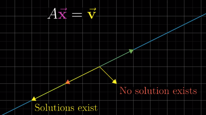
But this is not the case when $det(A) = 0$. In our example above, $\vec{v}$ definitely cannot be anything. For example, if $\vec{v}= \begin{bmatrix} 3 \\ -1 \end{bmatrix}$, we have:
$$\begin{eqnarray} x - y &=& 3 \\ 0x + 0y &=& -1 \end{eqnarray}$$
Which is nonsense.
If fact, the $y$ coordinate of $\vec{v}$ has to be 0; its $x$ coordinate can be anything. This it to say, $\vec{v}= \begin{bmatrix} c \\ 0 \end{bmatrix}$, and $c$ can be anything. We’ll have:
$$\begin{eqnarray} x - y &=& c \\ 0x + 0y &=& 0 \end{eqnarray}$$
Rank and Column space #
We keep using the terminology above. We have a $\vec{x}$, which, after applying a linear transformation of $A$, lands on $\vec{v}$.
We are most interested in knowing the coordinates of $\vec{x}$, because they will help us solve linear systems of equations. We compute the coordinates of $\vec{x}$ this way: $A^{-1}\vec{v}$.
Through the above example, we know that if $det(A) = 0$ and solutions exist, the coordinates of $\vec{x}$ must be on the line of $y = x - c$ (given that $\vec{v}= \begin{bmatrix} c \\ 0 \end{bmatrix}$).
However, if $det(A) \neq 0$, then the coordinates of $\vec{x}$ can bey anything on the x-y plane.
Therefore, the span of all possible $\vec{x}$ depend on $det(A)$: the span is smaller when $det(A) = 0$. We have a terminology for this difference: Rank.
Rank here is about a matrix or a linear transformation. Suppose we have countless input vectors ($\vec{x}$), and we apply $A=\begin{bmatrix} 1 & -1 \\ 0 & 0\end{bmatrix}$ to these input vectors. We’ll have output vectors ($A\vec{x}$). Aggregate all these output vectors. If the aggregated space is a line, we say $A$ has a rank of $1$ because the dimension of a line is $1$. If the aggregated space is 2D, we say $A$ has a rank of 2. Therefore, rank describes the number of dimensions in all the possible outputs of a linear transformation. In our example, for all vectors ($v$) in a 2D space, after applying $A = \begin{bmatrix} 1 & -1 \\ 0 & 0\end{bmatrix}$, $v$ become “projected” on the line of $y = 0$ in the $xy$ coordinates. Therefore, the $A$ has a rank of 1.
A related concept is column space: the span of the column vectors
. The column vectors of $A$ are $\begin{bmatrix} 1 \\ 0 \end{bmatrix}$ and $\begin{bmatrix} -1 \\ 0 \end{bmatrix}$. Therefore, the column space of $A$ is the space that can be reached by the linear combinations of $\begin{bmatrix} 1 \\ 0 \end{bmatrix}$ an$\begin{bmatrix} -1 \\ 0 \end{bmatrix}$, which is a 1D line. By the way, 3blue1brown defined column space of $A$ as the “set of all possible outputs of $A\vec{v}$”. I am not sure whether this definition is correct.
In fact, all the output vectors of $A$, i.e., $A\vec{x}$, are basically linear combinations of the two column vectors of $A$. Therefore, the rank of $A$ can also be defined as the dimension of its column space.
For a matrix $M$, if its rank is equal to the number of column vectors of $M$, we say $M$ has a full rank. In our example, the rank of $A$ is 1 but the its number of column vectors is 2. Therefore, $A$ does not have a full rank.
Another very important concept is null space of a matrix. In our example above, for all vectors ($v$) in a 2D space, after applying $A = \begin{bmatrix} 1 & -1 \\ 0 & 0\end{bmatrix}$, we will find that vectors along the line of $y=x$ become squashed into the origin, i.e., $(0, 0)$. We call vectors on the line of $y=x$ as the null space of $A$. Therefore, null space is the set of all vectors $v$ such that $A\times v =0$.
Lesson 8: nonsquare matrices as transformation between dimensions #
By now, we know what $\begin{bmatrix} 1 & -1 \\ 0 & 0\end{bmatrix}$ and $\begin{bmatrix} 6 & 6 & 6 \\ 33 & 44 & 55 \\ 6 & 10 & 14\end{bmatrix}$ mean. We know how the space is being transformed by these linear transformations, or, matrices. But how about nonsquare matrices?
For example, what does a $3 \times 2$ matrix mean? We know that a $3 \times 3$ matrix mean manipulating a 3D space, i.e., transforming a 3D vector into another 3D vector. But we don’t know what a $3 \times 2$ matrix means.
Let’s look at an example.
$$B = \begin{bmatrix} 2 & 0 \\ -1 & 1 \\-2 & 1\end{bmatrix}$$
This $3 \times 2$ matrix mean mapping 2D vectors onto a 3D space.
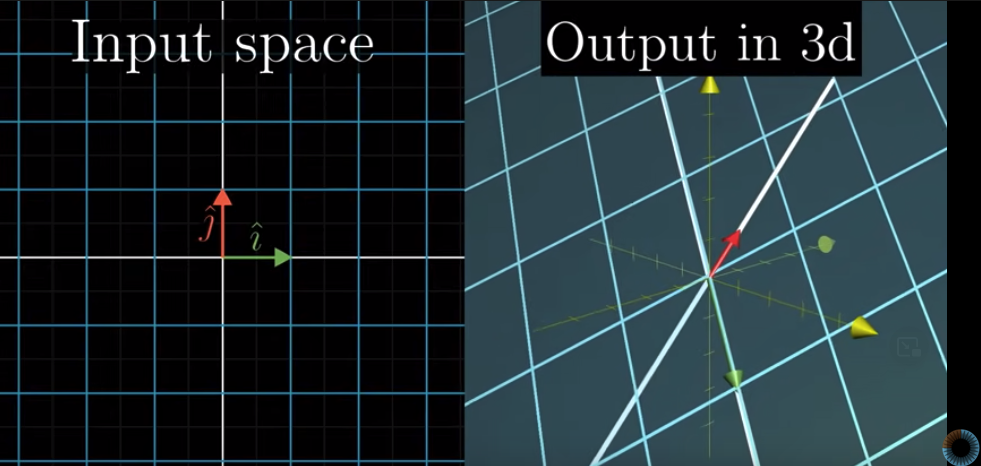
$\begin{bmatrix} 2 \\ -1 \\-2\end{bmatrix}$ is where the Transformed $\hat{i}$ lands and $\begin{bmatrix} 0 \\ 1 \\ 1\end{bmatrix}$ is where the Transformed $\hat{j}$ lands.
Note that the column space of $B$ is a 2D plane slicing through the origin in the 3D space. Therefore, its rank is 2. Because the rank is equal to the number of column vectors, $B$ is still full rank.
Likewise, a $2 \times 3$ matrix means mapping a 3D vector onto a 2D space, for example:
$$C = \begin{bmatrix} 3 & 1 & 4 \\ 1 & 5 & 9 \end{bmatrix}$$
The three vectors here represent the transformed $\hat{i}$, $\hat{j}$, and $\hat{k}$, respectively. If we have a three-dimensional vector, say $\begin{bmatrix} 1 \\ 1 \\1\end{bmatrix}$, it will become $\begin{bmatrix} 8 \\15 \end{bmatrix}$ in the 2D space after applying $C$.
In sum, a $m \times n$ matrix indicates transforming $n$-dimensional space to $m$-dimensional.
Lesson 9: dot products and duality #
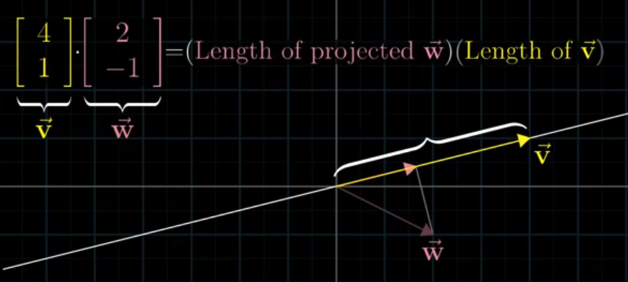
Dot product is traditionally described as projecting $\vec{w}$ onto $\vec{v}$. The length of $\vec{v}$ times the length of projected $\vec{w}$ is the dot project the two vectors.
We compute dot product this way:
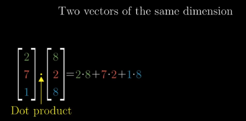
According to how dot product is calculated, it is easy to understand, algebraically, that the order of the two vectors does not matter. But how to understand it geometrically?
We can first consider two vectors of the same length:
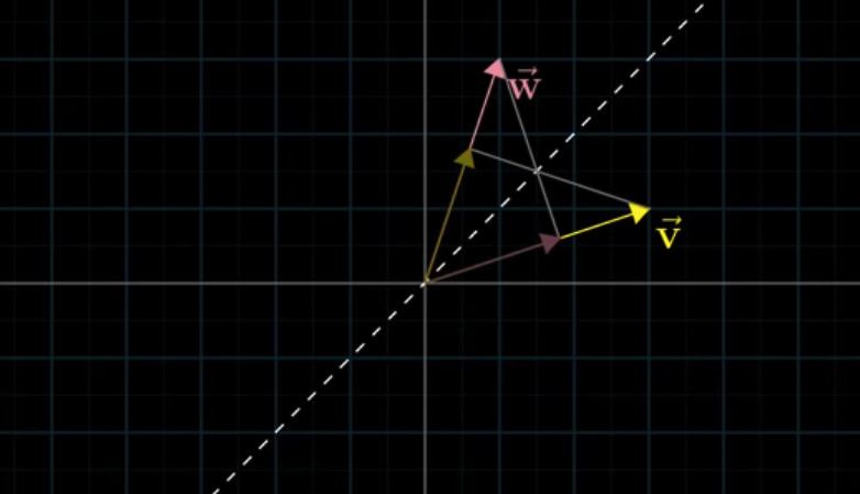
It is easy to understand in this case that the order does not matter. But what if the vectors are of different lengths? For example, what if $\vec{v}$ becomes $2\vec{v}$?
If $\vec{v}$ becomes $2\vec{v}$, the projected length of $\vec{w}$ does not change, so the result is two times the original result:
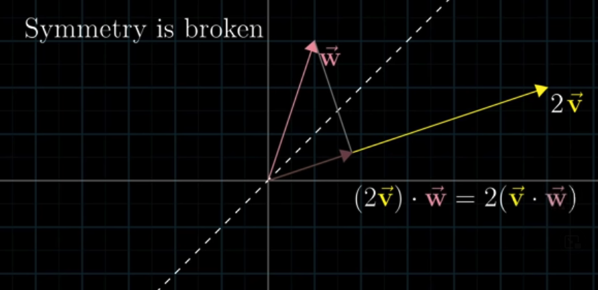
Similarly, the projected length of $2\vec{v}$ will be two times the projected length of $\vec{v}$. The result is, again, two times the original result:
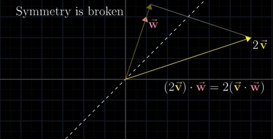
This is why the order does not matter.
Then, one important question is: Why on earth is dot project related to projection?
That’s a good question.
I don’t think 3blue1brown successfully answered this question. In the following, I’ll provide an answer inspired by the post of About Vector Projection by ParkJaJay.
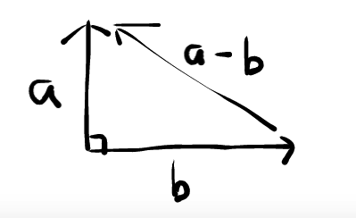
In the triangle below, if $\theta\neq90^o$, we have this:
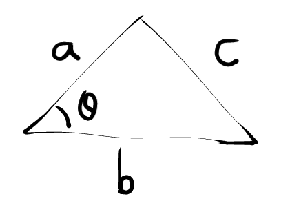
$$c^2 = a^2 + b^2 - 2ab\cos\theta$$
Also, when one vector is dotted by itself, the result will be the square of its length.
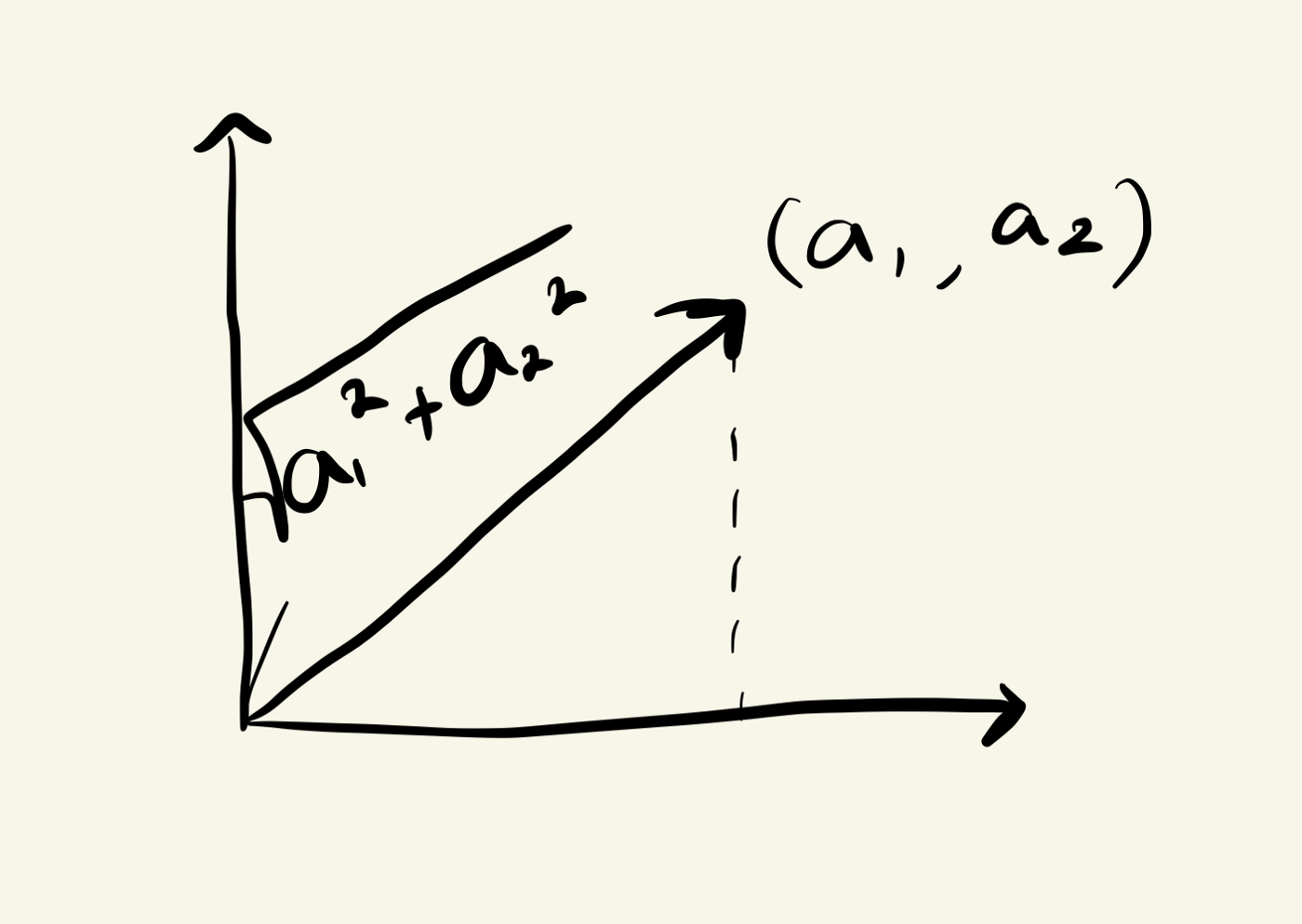
(Image by ParkJaJay)
$$\vec{a} \cdot \vec{a} = a_1^2 + a_2^2 = ||\vec{a}||^2$$
In the following, we have:
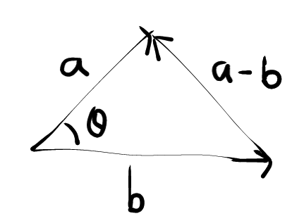
$$||\vec{a}-\vec{b}||^2 = ||\vec{a}||^2 + ||\vec{b}||^2 - 2||\vec{a}||||\vec{b}||\cos\theta$$
We also have:
$$||\vec{a}-\vec{b}||^2 = (\vec{a}-\vec{b}) \cdot (\vec{a} - \vec{b}) = \vec{a}^2 + \vec{b}^2 - 2\vec{a}\cdot\vec{b} = ||\vec{a}||^2 + ||\vec{b}||^2 - 2\vec{a}\cdot\vec{b}$$
Combine the abveo two, we have:
$$\vec{a}\cdot\vec{b} = ||\vec{a}||||\vec{b}||\cos\theta$$
If $\theta = 90^o$, we have
$$||\vec{a}-\vec{b}||^2 = ||\vec{a}||^2 + ||\vec{b}||^2$$
So we have:
$$||\vec{a}||^2 + ||\vec{b}||^2 = ||\vec{a}||^2 + ||\vec{b}||^2 - 2\vec{a}\cdot\vec{b}$$
So:
$$2\vec{a}\cdot\vec{b} = 0$$
This is how the dot product of two vectors is related to vector projection. This is also why a positive dot product indicates that the two vectors are pointing to generally the same direction, a negative dot product indicates different directions, and the dot product of 0 means the two vectors are perpendicular to each other.
3blue1brown rightly pointed it out that the dot product of two vectors is related to a linear transformation:
$$\begin{bmatrix} a_1 \\a_2 \end{bmatrix}\cdot \begin{bmatrix} b_1 \\b_2 \end{bmatrix} = \begin{bmatrix} a_1&a_2\end{bmatrix} \begin{bmatrix} b_1 \\b_2 \end{bmatrix} = a_1b_1 + a_2b_2$$
Therefore, perfoming a linear transformation denoted by $\begin{bmatrix} a_1&a_2\end{bmatrix}$ is the same as taking a dot product with $\begin{bmatrix} a_1 \\a_2 \end{bmatrix}$.
Lesson 10 & 11: Cross Product #
The cross product of two vectors $\vec{v}$ and $\vec{w}$ in 3d space is defined this way:
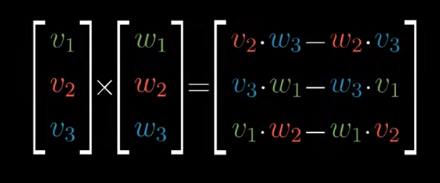
The outcome vector, i.e., $\begin{bmatrix} v_2 \cdot w_3 - w_2 \cdot v_3 \\ v_3 \cdot w_1 - w_3 \cdot v_1 \\ v_1 \cdot w_2 - w_1 \cdot v_2\end{bmatrix}$ has the following properties:
- It is perpendicular to both
$\vec{v}$and$\vec{w}$ - Its direction follows the right hand rule:
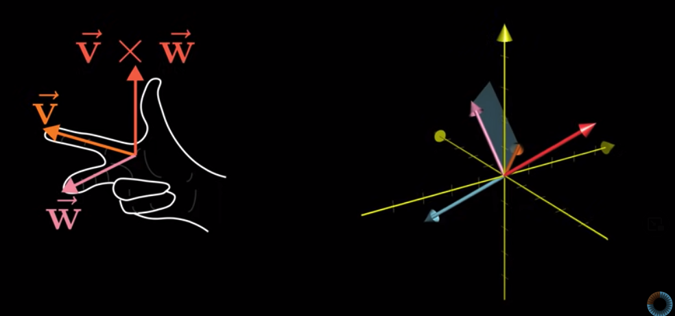
- Its length is equal to the area of the parallelogram of
$\vec{v}$and$\vec{w}$
BUT, WHY?
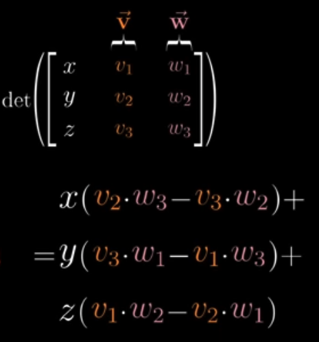
To understand why, let’s first think there is a variable vector in the 3d space: $\vec{m} = \begin{bmatrix} x \\y\\z \end{bmatrix}$. The volume of the parallelepiped of $\vec{m}$, $\vec{v}$ and $\vec{w}$ is its determinant:
How come?
This is because for a 3 by 3 matrix, its determinant is calculated this way:
$$det \Biggl(\begin{bmatrix} a & b & c \\d & e & f \\g & h &i \end{bmatrix}\Biggl) = aei + bfg + cdh - ceg - afh - bdi$$
The output of this determinant, or volume, calculation, is a number. Since $\vec{v}$ and $\vec{w}$ are known, the coeffficents for $x$, $y$, and $z$ are also fixed. Therefore, the calculation of the determinant is just like mapping $\vec{m}$ onto the number line:
$$\begin{bmatrix} p_1 & p_2 & p_3 \end{bmatrix} \begin{bmatrix} x \\y\\z \end{bmatrix}$$
From Lesson 9, we know that this is equal to taking a dot product with $\vec{p} = \begin{bmatrix} p_1 \\p_2\\p_3 \end{bmatrix}$:
$$\begin{bmatrix} p_1 & p_2 & p_3 \end{bmatrix} \begin{bmatrix} x \\y\\z \end{bmatrix} = \begin{bmatrix} p_1 \\p_2\\p_3 \end{bmatrix} \cdot \begin{bmatrix} x \\y\\z \end{bmatrix} = det\Biggl(\begin{bmatrix} x & v_1 & w_1 \\y & v_2 & w_2 \\z & v_3 &w_3 \end{bmatrix} \Biggl)$$
So we have:
$$\vec{p} = \begin{bmatrix} p_1 \\p_2\\p_3 \end{bmatrix} = \begin{bmatrix} v_2 \cdot w_3 - w_2 \cdot v_3 \\ v_3 \cdot w_1 - w_3 \cdot v_1 \\ v_1 \cdot w_2 - w_1 \cdot v_2\end{bmatrix}$$
Let’s say the area of the parallelogram of $\vec{v}$ and $\vec{w}$ is $a$, and the length of the component of $\vec{m}$ perpandicular to $\vec{v}$ and $\vec{w}$ is $c$. The volume of the parallelepiped of $\vec{m}$, $\vec{v}$ and $\vec{w}$ should be $a \times c$:
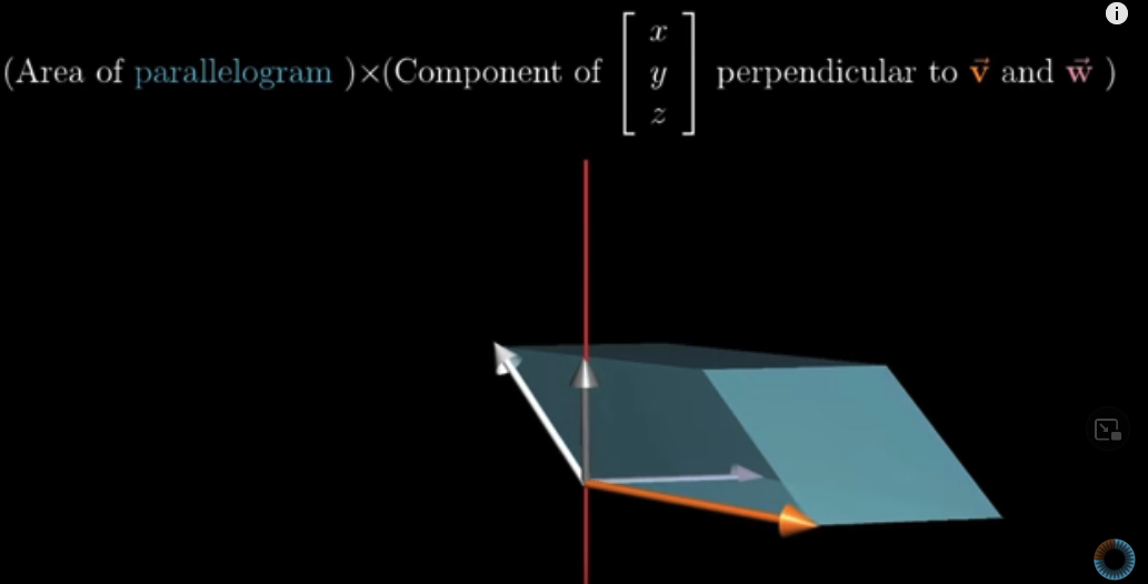
If $\vec{p}$ is perpendicular to both $\vec{v}$ and $\vec{w}$ and its length is equal to the area of the parallelogram of $\vec{v}$ and $\vec{w}$ , i.e., $a$, then the dot product of $\vec{m}$ and $\vec{p}$ is the length of $\vec{p}$, which is $a$, times the length of $\vec{m}$ projected on $\vec{p}$, which is equal to $c$: $a \times c$. This is also the volume of the parallelepiped of $\vec{m}$, $\vec{v}$ and $\vec{w}$.
$\vec{p}$ is the cross product of $\vec{v}$ and $\vec{w}$. That is why the cross product of $\vec{v}$ and $\vec{w}$ has the above mentioned properties.
Lesson 12: Cramer’s rule #
In Chapter 7, we talked about how linear algebra is useful for solving linear systems of equations through calculating the inverse matrix.
Let’s first review what we have learned.
Suppose we have this linear system of equation:
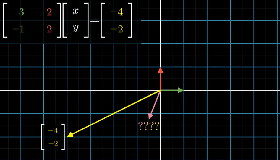
$$ \displaylines{3x + 2y = -4 \\ -x + 2y = -2} $$
The problem can be restated this way: we know a linear transformation: $\begin{bmatrix} 3 & 2\\ -1 & 2\end{bmatrix}$, and we know the output vector: $\begin{bmatrix} -4 \\-2 \end{bmatrix}$. We want to know what the input vector is: $\begin{bmatrix} x \\y \end{bmatrix}$.
$$\begin{bmatrix} 3 & 2\\ -1 & 2\end{bmatrix} \begin{bmatrix} x \\y \end{bmatrix} = \begin{bmatrix} 3 \\-1 \end{bmatrix} x + \begin{bmatrix} 2 \\2 \end{bmatrix} y = \begin{bmatrix} -4 \\-2 \end{bmatrix}$$
To know what the input vector $\begin{bmatrix} x \\y \end{bmatrix}$ is, we calculate the inverse matrix of $\begin{bmatrix} 3 & 2\\ -1 & 2\end{bmatrix}$, denoted as $A^{-1}$. Then the input vector will be the result of applying this inverse matrix to the output vector:
$$\begin{bmatrix} x \\y \end{bmatrix} = A^{-1}\begin{bmatrix} -4 \\-2 \end{bmatrix}$$
The drawback of this method is that it’s difficult to calculate the inverse matrix by hand.
A simpler way is the Cramer’s rule.
Let’s take another example here:
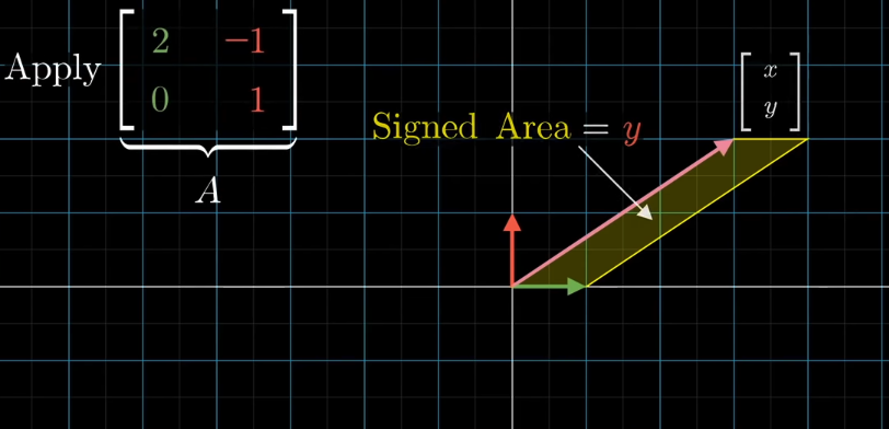
$$ \displaylines{2x - y = 4 \\ 0x + y = 2} $$
The most important idea behind Cramer’s rule is the determinant. The input vector is $\begin{bmatrix} x \\y \end{bmatrix}$ , and the area of the parallelogram made up of the input vector and $\hat{x}$ is $y$, because the length of $\hat{x}$ is 1.
The point here is that after applying $A$, all the areas will scale up or down by the same number, which is $det(A)$. Therefore, the area of the parallelogram made up of the Transformed $\hat{x}$ and the output vector $\begin{bmatrix} -4 \\-2 \end{bmatrix}$ is $det(A)y$.
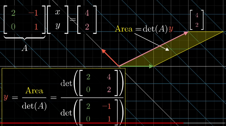
So if we know the area parallelogram made up of the Transformed $\hat{x}$ and the output vector, denoted as $Area$, we can calculate $y$ by:
$$y = \frac{Area}{det(A)}$$
And we know $Area$ because we know the coordinate of Transformed $\hat{x}$ and the output vector:
$$Area = det\Biggl(\begin{bmatrix} 2 & 4\\ 0 & 2\end{bmatrix}\Biggl) = 2*2 - 0*4 = 4$$
If you don’t know how the above calcultion works, brush up on the chapter of determinants. Just imagine, if the output vector is the Transformed $\hat{y}$, what will be the determinant? That’s how we calculate the above $Area$.
And we know that
$$det(A) = det\Biggl(\begin{bmatrix} 2 & -1\\ 0 & 1\end{bmatrix}\Biggl) = 2*1 - 0*-1 = 2$$
Therefore, we have $y = \frac{4}{2} = 2$. And indeed, $y = 2$.
The same is for the calculation of $x$. One thing to note that when calculating the area made up of the transformed $\hat{x}$ and the output vector, the first column should be the transformed $\hat{x}$ whereas when calculating the area made up of the transformed $\hat{y}$ and the output vector, the first column should be the output vector.
What about three dimensions?
$$ \displaylines{3x + 2y + 7z= -4 \\ 1x + 2y - 4z = -2 \\ 4x + 0y + 1z = 5} $$
This is the same as:
$$\begin{bmatrix} 3 & 2 & 7\\ 1 & 2 & -4 \\ 4 & 0 & 1\end{bmatrix} \begin{bmatrix} x \\y \\ z \end{bmatrix} = \begin{bmatrix} 3 \\1 \\4 \end{bmatrix} x + \begin{bmatrix} 2 \\2 \\0 \end{bmatrix} y + \begin{bmatrix} 7 \\ -4 \\1 \end{bmatrix} z = \begin{bmatrix} -4 \\-2 \\5 \end{bmatrix}$$
The volume of the parallelepiped made up of $\hat{x}$, $\hat{y}$, and the input vector is $z$. The determinant of $A$ is:
$$det\Biggl(\begin{bmatrix} 3 & 2 & 7\\ 1 & 2 & -4 \\ 4 & 0 & 1\end{bmatrix}\Biggl) = -84$$
The volume of $\hat{x}$, $\hat{y}$, and the output vector is:
$$det\Biggl(\begin{bmatrix} 3 & 2 & -4\\ 1 & 2 & -2 \\ 4 & 0 & 5\end{bmatrix}\Biggl) = 36$$
Therefore, we have:
$$z = \frac{36}{-84} = -\frac{3}{7}$$
We can calculate $x$, and $y$ in the same way.
Lesson 13: Change of basis #
A “coordinate system” translate vectors in to a set of numbers. In our standard coordinate system, $\hat{i}$ and $\hat{j}$ are called “basis vectors”.
But what if we use different basis vectors?
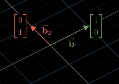
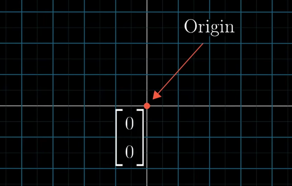
The same vector in space will be described differently if we use alternative basis vectors. Note that the origin is the same no matter what basis vectors you use.
Now that we can have different coordinate systems, how do we translate between them?
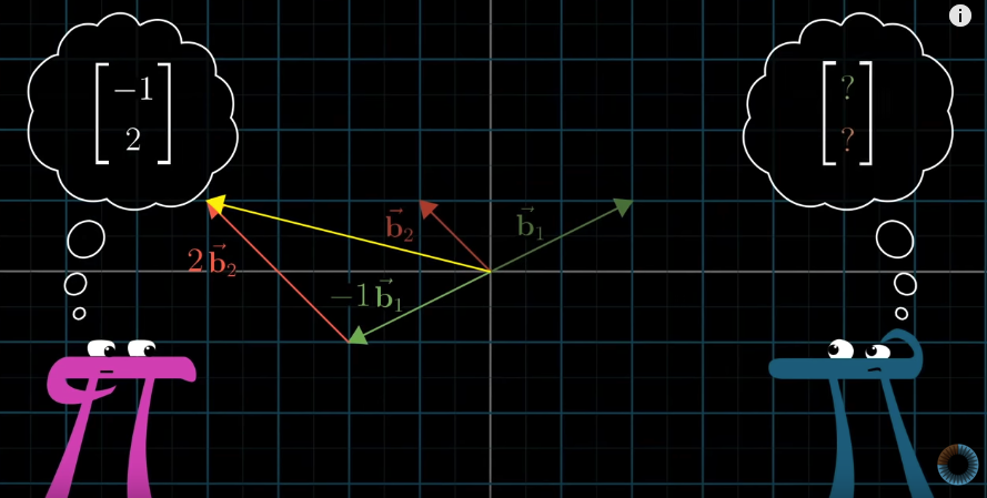
We can calculate it this way:
$$\vec{c} = -1\vec{b_1} + 2\vec{b_2} = -1 \begin{bmatrix} 2 \\1 \end{bmatrix}+ 2 \begin{bmatrix} -1 \\1 \end{bmatrix} = \begin{bmatrix} -4 \\1 \end{bmatrix}$$
This looks similar, right? In Chapter 3, we talked about linear transformation. The above calculation is the same as linear transformation. For any vector described in Jennifer’s world, $\vec{v} = \begin{bmatrix} x \\y \end{bmatrix}$, we apply the transformation of $\begin{bmatrix} 2 & -1 \\ 1 & 1 \end{bmatrix}$ to it, and the result will be how the output vector in Jennifer’s world is interpreted in our “standard” world.
To reiterate: we have a vector $\vec{v} = \begin{bmatrix} x \\y \end{bmatrix}$ described in Jennifer’s world. And we know that the basis vectors that Jennifer is using can be interpreted in our world: $\begin{bmatrix} 2 & -1 \\ 1 & 1 \end{bmatrix}$. To know what will be the coordinates of $\vec{v}$ in our language, we apply the linear transformation of $\begin{bmatrix} 2 & -1 \\ 1 & 1 \end{bmatrix}$ to $\vec{v}$.
Then, what if we have a vector $\vec{m} = \begin{bmatrix} x_m \\ y_m \end{bmatrix}$ described in our world, and we want to know how it will be described in Jennifer’s world? We calculate the inverse of the matrix of $\begin{bmatrix} 2 & -1 \\ 1 & 1 \end{bmatrix}$ and apply that inverse matrix to $\vec{m}$.
The inverse matrix will be $\begin{bmatrix} \frac{1}{3} & \frac{1}{3} \\ - \frac{1}{3} & \frac{2}{3} \end{bmatrix}$. Take the above example of $\vec{m} = \vec{v} = \begin{bmatrix} -4 \\1 \end{bmatrix}$. When we apply the inverse matrix to it, the result will be:
$$\vec{v} = \begin{bmatrix} -4 \\ 1 \end{bmatrix} \begin{bmatrix} \frac{1}{3} & \frac{1}{3} \\ - \frac{1}{3} & \frac{2}{3} \end{bmatrix} = -4 \begin{bmatrix} \frac{1}{3} \\ - \frac{1}{3} \end{bmatrix} + 1 \begin{bmatrix} \frac{1}{3} \\ \frac{2}{3} \end{bmatrix} = \begin{bmatrix} -1 \\ 2 \end{bmatrix}$$
Lesson 14: Eigenvectors and eigenvalues #
Eigenvectors are those that remain in their span after a linear transformation. Eigenvalues represent how much they are streched.
How to compute eigenvectors and eigenvalues then?
Let’s take a concrete example. Let’s say the linear transformation is $A = \begin{bmatrix} 2& 2\\ 1 & 3 \end{bmatrix}$. Let’s say $\vec{v}$ is one eigenvector, and $\lambda$ is the associated eigenvalue. Because the eigenvectors remain in its span, but streched, we have:
$$A\vec{v} = \lambda\vec{v}$$
We can insert an identity matrix to the right hand side: $\lambda \begin{bmatrix} 1 & 0 \\ 0 & 1 \end{bmatrix}\vec{v}$. This is because
$$\begin{bmatrix} 1 & 0 \\ 0 & 1 \end{bmatrix}\vec{v} = \vec{v}$$
Denoting the identity matrix as $I$, we have:
$$A\vec{v} - \lambda I \vec{v} = (A-\lambda I)\vec{v} = \vec{0}$$
Of course, this will be true if $\vec{v} = \vec{0}$, but we are not interested in this. We want non-zero solutions to $\vec{v}$. If $\vec{v}$ is a non-zero vector and after applying the linear transformation of $A - \lambda I$, it becomes a zero vector, it means $det(A - \lambda I) = 0$. That is to say:
$$det\Biggl(\begin{bmatrix} 2-\lambda & 2\\ 1 & 3- \lambda\end{bmatrix}\Biggl) = (2-\lambda)(3-\lambda)-2=0$$
So, $\lambda = 4$ or $1$. When $\lambda = 4$, we have:
$$(\begin{bmatrix} 2& 2\\ 1 & 3 \end{bmatrix} - 4 \begin{bmatrix} 1 & 0 \\ 0 & 1 \end{bmatrix}) \vec{v} = (\begin{bmatrix} -2&2\\ 1 & -1 \end{bmatrix})\vec{v}=\vec{0}$$
Suppose $\vec{v} = \begin{bmatrix} x\\ y \end{bmatrix}$, we have:
$$x\begin{bmatrix} -2\\ 1 \end{bmatrix} + y \begin{bmatrix} 2\\ -1 \end{bmatrix} = \begin{bmatrix} -2x + 2y\\ x-y \end{bmatrix} = \begin{bmatrix} 0\\ 0 \end{bmatrix} $$
So eigenvectors are along this line: $y=x$. The same procedure can be applied to compute the eigenvectors for when $\lambda = 1$.
Last modified on 2025-07-02 • Suggest an edit of this page