Understanding 3blue1brown Vidoes on Neural Networks

Lesson 1: what is a neural network #

It is easy for our brain to recognize handwritten digits, but when you are asked to write a program and let the computers be able to do the same thing, you’ll find it super difficult.

Neural networks have two elements: neurons and the links between them.

Think of a neuron as something that holds a number between 0 and 1.

The first step is that we have $28 \times 28 = 784$ neurons, each holding a number that represents the grayscale value of a corresponding pixel: 0 means black and 1 means white. This number is called an “activation”.

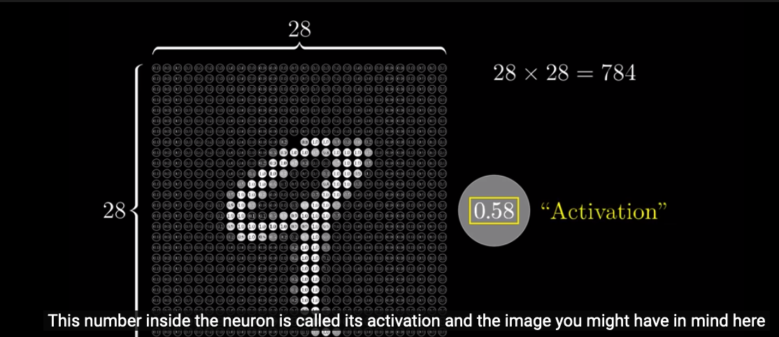
These 784 neurons are the first layer of our neural network.

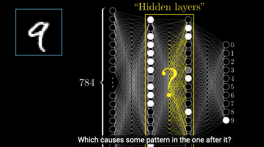
The last layer has 10 neurons, each represents a digit (from 0 to 9). The activation in each neuron represents how likely our system thinks this image correspondes to a given digit.

And in between, we have two hidden layers.

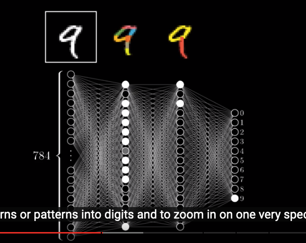
How this system works is that activation patterns in the first layer will cause some specific patterns in the 2nd layer, and then the pattern in 2nd layer causes specific patterns in the 3rd layer. The process goes on and on, until we reach the output layer. In the output layer, the neuron holding the largest number will be our system’s guess.

Then, the question is, why we need hidden layers and what these hidden layers do.

The way how our human brains recognize handwritten digits is that we parse the image into several parts. For example, 9 consists of a loop on top and a vertical line at the bottom and 8 consists of two loops stacked together.

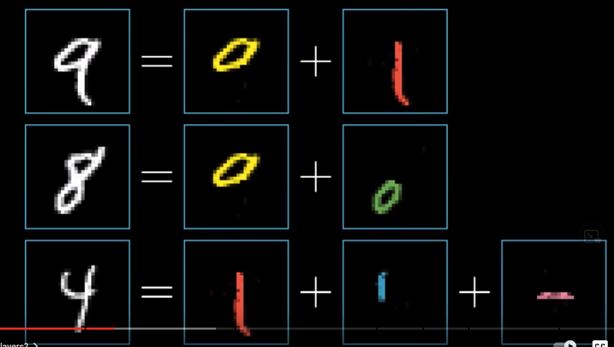
What we hope the hidden layers will do is that each neuron will represent a specific component. For example, in the 3rd layer, we hope that, one neuron represents an upper loop and another represents a lower vertical line. When our system is processing the image of 9, in the third layer, these two neurons will be very bright (because their activations will be close to one). Then, based on the combinations of these components in the third layer, the neurons in the output layer will have different activations (and the brightest one will be our system’s guess).

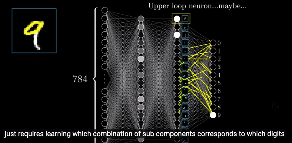
Then, the problem is, how do we recognize an upper loop or a lower vertical line ?

The task of recognizing a loop can be broken down into first recognizing some smaller edges.

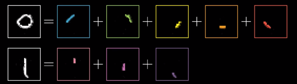
In the second layer, we hope that small edges will be recognized, and these recognized edges will light up certain neurons in the 3rd layer.

We will revisit whether our neural network actually does this but that’s the hope we have.

This layered structure is useful for all sorts of recognition taks, such as labelling images and speech recognition.

Weights #

Let’s go back to what the 2nd layer is doing. Let’s say we want to detect an upper horizontal line (or any other pattern).

What we have in the first layer is 784 neurons (with activiations) each representing a pixel in the image. Let’s say the one neuron in the above image in the 2nd layer is for the upper horizontal line we want to detect. Hereafter, we call this neuron as that neuron. What we want is that different patterns in the 1st layer will result in different activations for that neuron in the 2nd layer. How can we do that?

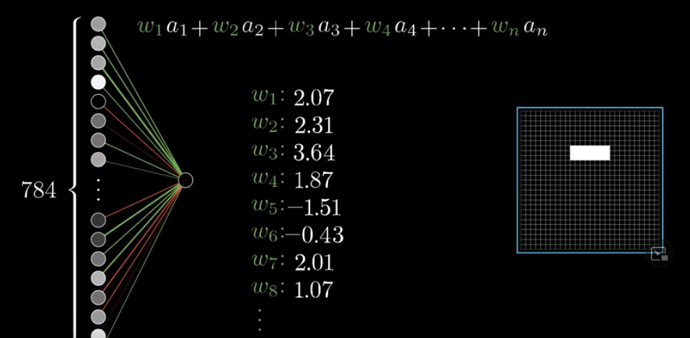
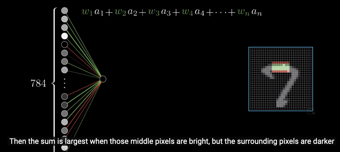
We should notice that each neuron in the 1st layer represnets a pixel in the image. Because the horizontal line we want to detect is located in the upper middle, the neurons in the 1st layer corresponding to this area will have more influences on the activation of that neuron in the 2nd layer. That’s why we give different weights to the connections between each neuron in the 1st layer and that neuron in the 2nd layer.

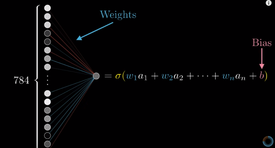
When examining an image, for each neuron in the 1st layer, we compute the product of the weight we assigned to it and its activation. We then sum up these products. This sum is the activation of that neuron in the 2nd layer.

To make sure that the pattern is a pattern of itself, rather than a part of a larger pattern, we assign negative weights to pixels surrounding the area we care about. This way, if the pattern is a a pattern of itself, the activations of neurons corresponding to these surrounding areas will be small (because there is nothing in there), and thus the sum of the products described above will be large (as their weights are negative). On the other hand, if the pattern is a part of a larger pattern, then the activations of neurons corresponding to these surrounding areas will be big, and thus the sum will be smaller.

Note that the wegithed sum computed like above is not necessary between 0 and 1 (most of the time, it isn’t). Since this weighted sum is the activation for that neuron in the 2nd layer, we want it to be between 0 and 1. How to do that?

We can use the Sigmoid function.

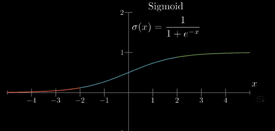
With Sigmoid function, very negative numbers are transformed to a number close to 0 and very positive numbers to numbers close to 1.

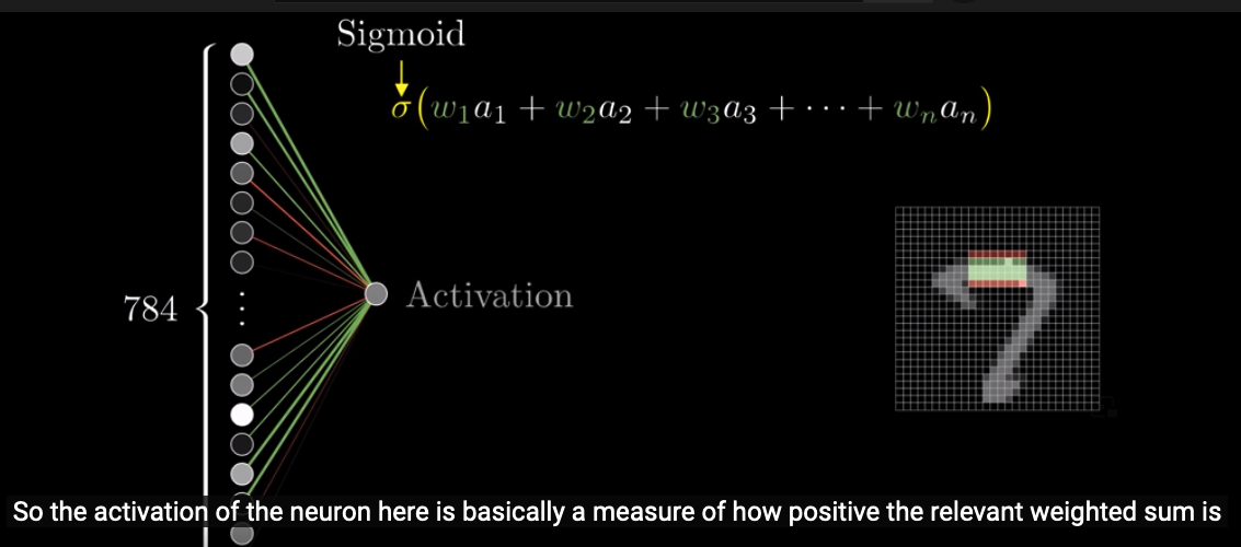
This way, what the activation of that neuron in the 2nd layer measures is how positive the weighted sum is:

To be more robust, we can set a threshold for the activation. For example, we want the activation to be above 0 only when the weighted sum is bigger than 10. This is easy to implement. We can simply add a $-10$ at the end of the input of the Sigmoid function:

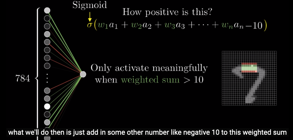
That number, $-10$ in our case, is called a “bias”. More specifically, a bias for inactivity.

To recap, weights tell us what pixel pattern this neuron in the second layer is picking up on and the bias tells us how big the weighted sum needs to be before we “light up” the neuron.

Note that we have been talking about only one neuron (that picks up on the pattern of a horizontal bar) in the 2nd layer. But there are 16 neurons in the 2nd layer. For each neuron in the 1st layer, their associated weights are dependent on its connection to the neuron in the 2nd layer. That is to say, for example, the weight of Neuron A1 in the 1st layer is $.25$ when we are talking about Neuron B1 in the 2nd layer. However, the weight of Neuron A1 changes to $.5$ when we are talking about Neuron B2 in the 2nd layer.

Also, each neuron in the 2nd layer will have its own bias for inactivity.

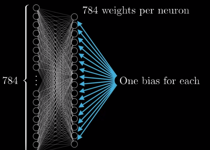
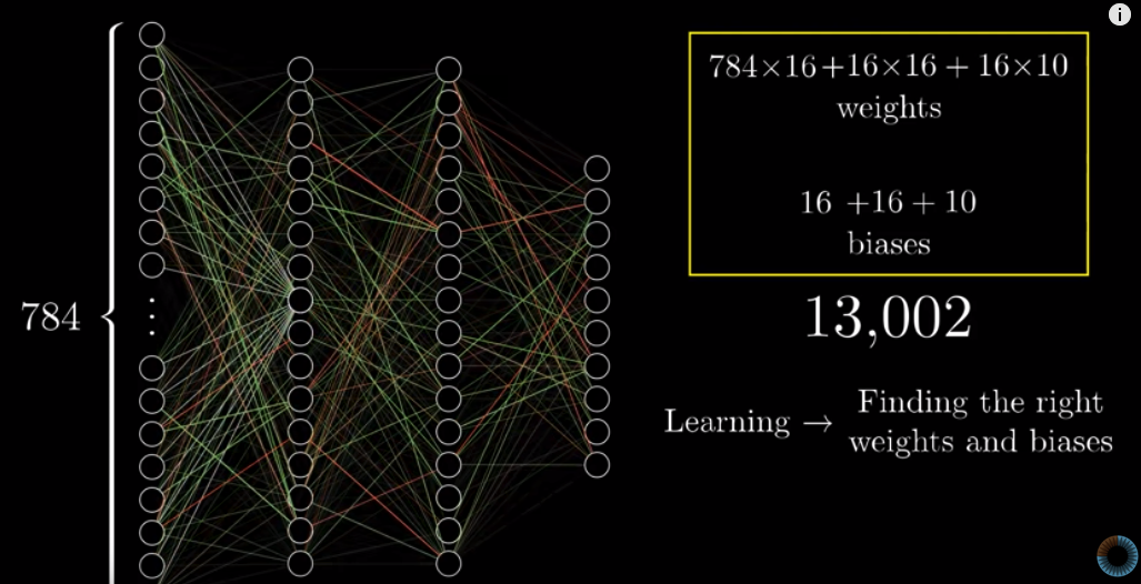
Therefore, if we only examine the 1st and the 2nd layer, we have $784 \times 16$ weights and 16 biases. When we examine the whole neural network, we have over 13K weights and biases.

These weights and biases are parameters we are able to tweak. Learning is all about finding the appropriate weights and biases.

Recap #

To recap, each neuron in one layer is connected to each neuron in the next layer. The weights represent the strength of each connection, and the bias represents whether a neuron in the next layer tends to be active or inactive.

Mathematical representation #

The way we calculate the activation of each neuron in the 2nd layer is that we calculate the weighted sum of all neurons in the 1st layer, then consider the bias, and then apply Sigmoid function to this result. But how can we represent this procedure mathematically?

Suppose we have $n$ neurons in the first layer and $k$ neurons in the next layer. The first step of the above procedure can be expressed as the multiplication of a $k \times n$ matrix (i.e, $n$ weights for each one of the $k$ neurons in the next layer) and a $n \times 1$ matrix (i.e., $n$ activations in the first layer). The result is a $k \times 1$ matrix.

In the $n \times 1$ matrix, each row is the activation of a neuron in the first layer. In the $k \times n$ matrix, each row is all the weights of the 1st layer when we consider a specific neuron in the next layer.

To consider biases for inactivity, we add a $k \times 1$ matrix, where each row represents a bias for a particular neuron in the next layer. And then we apply a Sigmoid function.

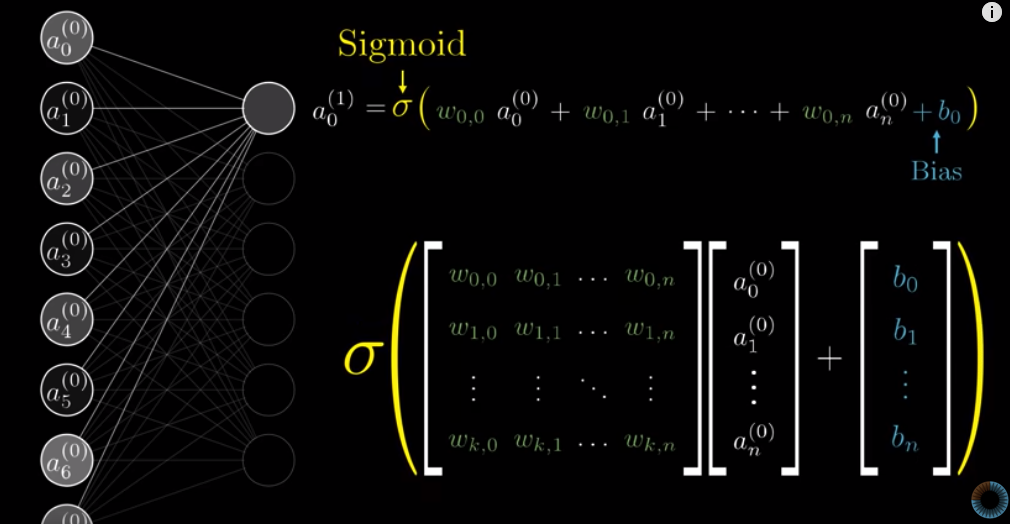
Note that there are some issues with the above illustration by 3blue1brown.

• First, the number of rows in the first matrix seems to be $n$, but this is incorrect. It should be $k$, i.e., the number of neurons in the next layer.
• Second, the bias vector should be from $b_0$ to $b_k$ rather than to $b_n$.

The final result will be a $k \times 1$ matrix, where each row is the activation for each neuron in the next layer.

The vector of activations of the 2nd layer can be expressed as:

$$a^{(1)} = \sigma(Wa^{(0)} + b)$$

where $a^{(n)}$ represents the vector of activiations in the $n^{th}$ layer, $W$ represents the $k \times n$ matrix of weights, $\sigma$ represents the Sigmoid function, and $b$ represents the bias vector.

To express it in Python:

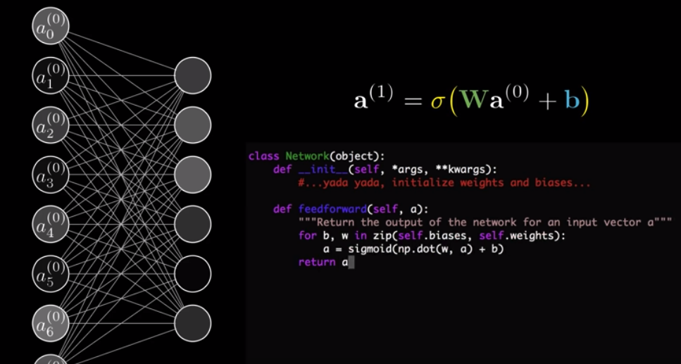
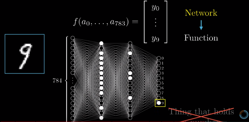
We earlier said that we can consider each neuron as something that holds a number. This number is dependent on the activations and weights of neurons in the previous layer and also the bias for the neuron we are considering. Therefore, it is more accurate to consider a neuron as a fuction, taking in outputs of all neurons in the previous layer and spits out a number between $0$ and $1$.

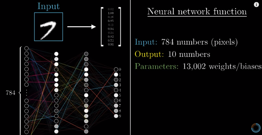
In fact, we can consider the entire neural network as a function: taking in activations in the first layer and spits out 10 numbers as an output, with over 13K weights + baises being the parameters.

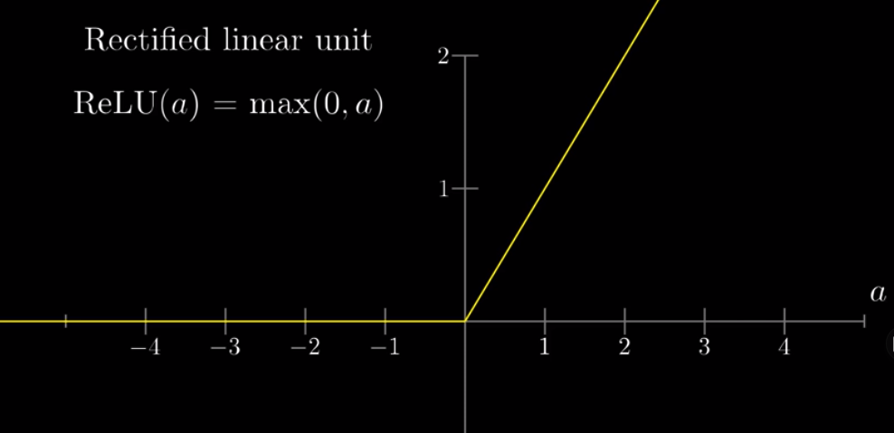
At the end of the video, it is noted that nowadays, people rarely use Sigmoid functions to squish the weighted sum into a number between 0 and 1. Instead, people use the ReLU function, which is more similar to how neurons actually work. ReLU stands for rectified linear unit.

ReLU (a) = max (0, a)

Lesson 2: Gradient descent, how neural networks learn #

We train our neural network with a buch of training data which consists of images and the correct labels. Then our neural network will adjust its over 13K parameters, i.e., weights and biases, to maximize its performance. After the training, we test the neural network with more labelled data, i.e., the test data.

To start off, we randomize every weight and bias. The result must be horrible since most likely it will be different from the true outcome, i.e., 10 numbers in the last layer.

We need, therefore, to know how different is our result from the correct answer. We call this as a cost function, meaning the “cost” of this difference. You can also call it a loss function .

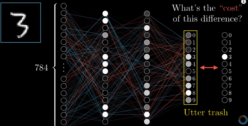
This is how we calculate the cost: the sum of squares of the difference between each activation in the random result and its associated correct result.

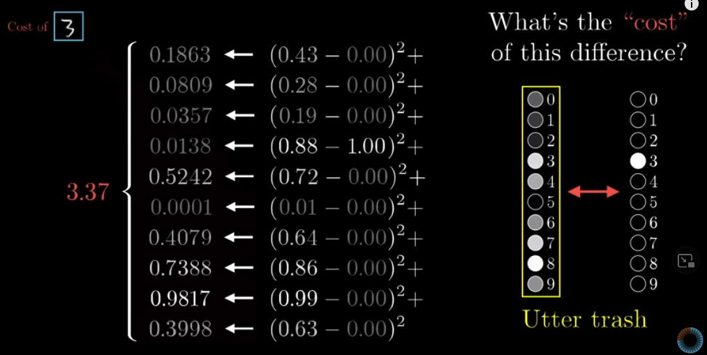
We call this the cost of a training example. The cost is small when the system’s guess is close to the actual result and big when the guess is totally off target.

That cost is a measure of the accuracy of a training example. But how to measure the accuracy of our entire neural network ? We take the average of cost of all the training data.

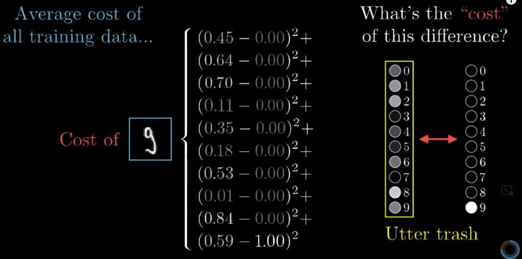
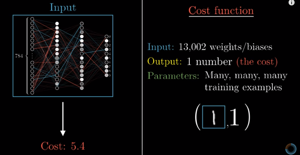
The cost for a given neural network is actually a function: it takes in the result our system guesses and also the actual result, and spits out a number as an output, which is the cost of this neural network.

In the video, 3Blue1Brown says that the cost function takes in 13K weights + biases, spits out a number that is the cost, and that training examples are the parameters. This interpretation is also reasonable.

In a function, for example, $y = 2x^2 -1$, the input, $x$ in this example, is something that is always changing. Parameters, $2$ and $1$ in our example, are fixed. The output, $y$ is depent on $x$, and that is why it is called a dependent variable, or an outcome variable.

In terms of cost, no matter whether we are talking about a cost for a single training example, or the average cost for the entire neural network, what are fixed are the training examples. They are the parameters. The output is the cost. Given the training examples, what is the output depent on ? It is dependent on the over 13K weights and biases that we can adjust.

Essentially, the cost of our neural network is the errors that our model made (simplilearn.com ).

It is therefore our job, or our computer’s job, to minimize the cost, or the errors, by tweaking the over 13K weights and biases. The heart of machine learning to minimize the cost function. However, that’s not a trivial task!

The process of finding local minimum for the cost function is called gradient descent, which involves calculus. It is beyond my ability to understand since I have never learnt calculus before. You may check out this explanation .

Now, go back to our intial hope: we hope that the 2nd and 3rd layer is picking up on some patterns. Specifically, we hope that the 2nd layer can identify small edges and the 3rd layer can identify larger components. The question is, are they really doing it ?

The answer is, at least in our example, NO.

Let’s look at the weights of all the connections between the 1st and the 2nd layer. We project these to a $28 \times 28$ matrix. Recall that the wegiths represent the strengths of the connections. If the 2nd layer is actually picking up small edges, there should be some pattern in the weights. But they are not.

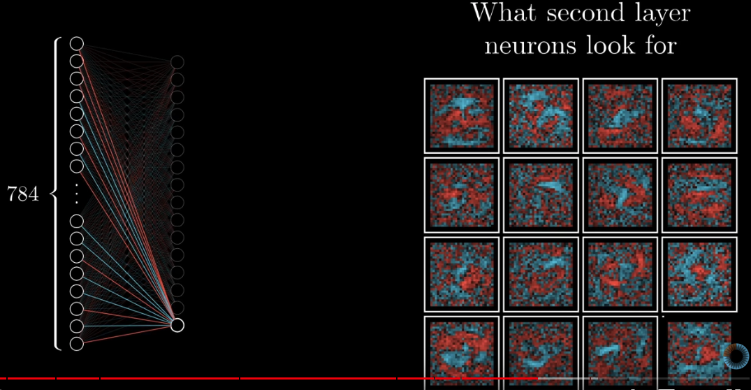
The above picture shows these weights. Blue presents positive weights and red presents negative weights. We can say that the pixels with postive weights are what the 2nd layer is looking for. We can see that there are no patterns for positive weights.

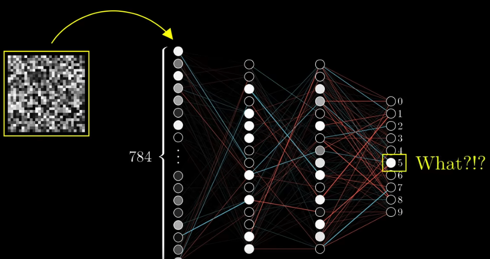
The problem with this is that even if we give the system a random image, which does not show any handwritten digit, the system will still give us an answer confidently, which is obviously incorrect.

These resources are recommended at the end of the video:

• Neural Networks and Deep Learning by Michael Nielsen
• Neural Networks, Manifolds, and Topology on colah’s blog
• Why Momentum Really Works

Lesson 3, Backpropagation #

Backpropagation is an algorithm to calculat the gradients for all the wegiths and baises. The bigger a gradient is, the more influence the corresponding weight or bias has on the cost.

The purpose of doing backpropagation is to minimize the cost for the neural network. That minimization is dependent on all training examples. This is hard to comprehend. For this lesson, we focus on only one training example, looking at how backpropagation works in that case.

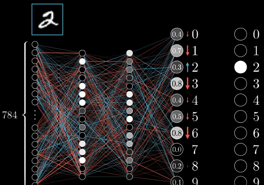
Take the image of a handwritten $2$ as an example. In the output layer, we want the activiation of that neuron (Let’s call it $n_{out2}$) corresponding to $2$ to be $1.0$ and activiation of all other neurons to be $0.0$. Therefore, we want to increase the activation of $n_{out2}$, and decrease the activation of other neurons. The change of activations include both direction and quantity. For example, if the activation of the neuron corresponding to $3$ is previously $0.9$, then we want it to decrease a lot. The activation of the neuron corresponding to $8$ was $0.2$, so we only need it to decrease a little bit.

We, however, are not able to directly change the activations in the output layer. We can achieve this goal by adjust the weights and biases. Let’s first take $n_{out2}$ as an example. We want to increase its activation. Recall that one neuron’s activation is calculated this way:

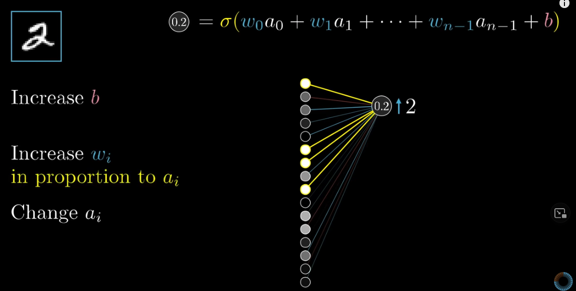
To increase the activation of $n_{out2}$, the first choise, obviously, is to increase the biase, $b$.

The second option is to increase the weights. All activations in the previous layer is equal to or bigger than $0$. Therefore, to make the activation $n_{out2}$ large, we want all weights to be positive. Also, note that brighter neurons (those with higher activations) have bigger impacts on the activation of $n_{out2}$. Therefore, we want the increases in weights connecting those brigher neurons to be larger than those in weight connecting dimmer neurons.

This makes sense. Recall that the weights represents the strengths between connections. If a neuron in the third layer has a higher activation when seeing an image of $2$, then it indicates that that neuron, or more specifically, the pattern that neuron picks up, is more related to $2$. Then, its connection with the neuron in the output layer representing $2$, must be stronger.

The third option is to change the activation in the third layer. For neurons with positive weights, we want their activiations to increase. For neurons with negative weights, we want their activations to decrease. The amount of change should be proportional to the weights.

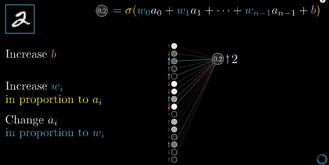
Of course, we cannot change the activations directly. But if we know in which direction and by how much we want the activations in the third layer to change, we can accordingly change the weights and baises with the 2nd layer. That is exactly what backpropagation is supposed to do.

Now, you may wonder. Hmm, then we only need to change the weights associated with the brighter neurons to be $+ \infty$, and we also want the activations with positive weights to increase to $1$. This way, the activation of $n_{out2}$ will be large.

No. But why ?

Because we are not only consider $n_{out2}$, but also $n_{out1}$, $n_{out2}$, … Each of these neurons has its own thoughts about how weights and activations in the third layer should change.

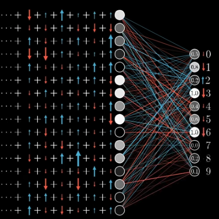
The desired changes to the weights, biases, and activations are the sum of considerations by all the activations in the output layer.

Once, we get the desired change for each activation in the 2nd but last layer, we propagate backwards and change the weights, baises, and activations in the 3rd but last layer.

We mention we want to change the activations in the 3rd, and 2nd layer. But we are not actually going to change, nor we could. We just use those desired changes to infer how we want to change the weights and baises.

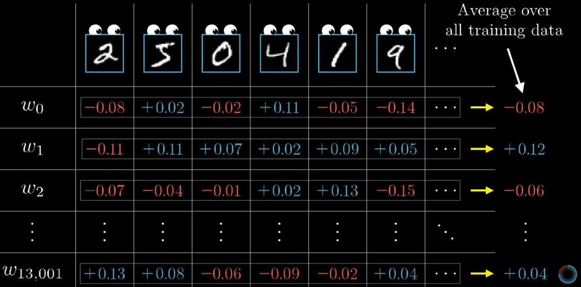
Once the back propagation is over, we know in which direction, and by how much, we want to nodge all the 13K weights and biases. However, keep in mind that those changes are the result of considering only one training example. But we have tens of thousands of training examples. What we do is to consider all those desired changes for each weight and bias and take the average.

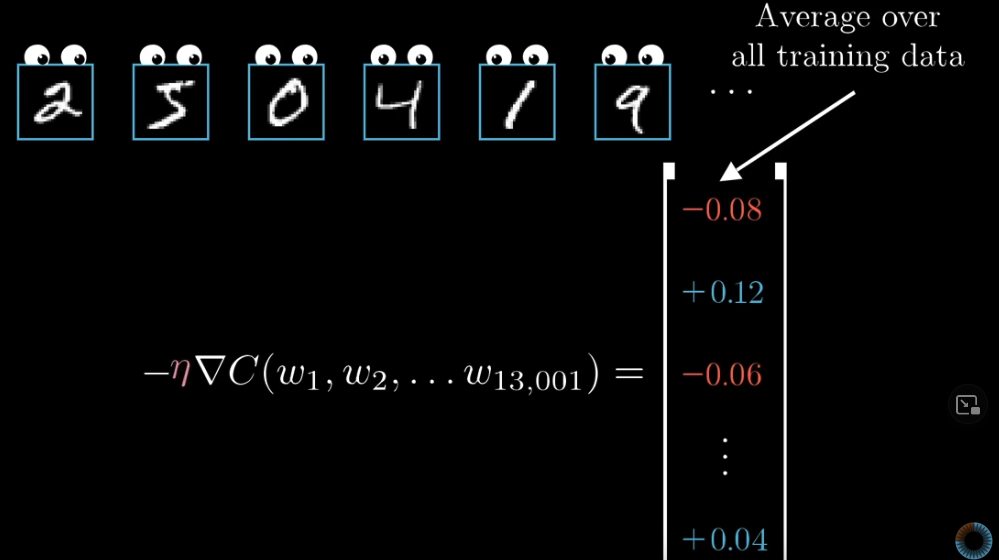
These averaged desired changes are very close to the vector of gradients we talked about earlier. We can at least consider them as something proportional to the gradients.

It is computationally expensive to add up the impact of each training example. To make the process more efficient, we normally randomly shuffle our training dataset, and devide them into mini-batches. For example, if the whole training data consists of 10K examples, we can have 100 mini-batches each containing 100 training examples. For each mini-batch, we calculate the average desired changes for each weight and bias. The results won’t be perfect, but each mini-batch gives us a rough sense of what the final gradients should be. This makes it easier for computers. This technique is called Stochastic gradient descent.

Last modified on 2022-10-30